Chapter 8  :  The Standard Cost Accounting System Part 2: Journal Entries, Cost Variances, And Reports

Learning Objectives

After studying this chapter, you should be able to:

1. Discuss the role of a standard cost accounting system (SCAS) in responsibility accounting.

2. Explain the meaning of a cost variance, and calculate and interpret the variable costs' spending vari­ances.

3. Calculate and interpret the variable costs' usage variances.

4. Calculate and interpret the fixed overhead variances.

5. Prepare the journal entries for an SCAS, and the cost variance report.

6. Design a high-quality SCAS with management reports useful for operational control and performance evaluation.

6. Prepare a list of attributes needed in a relational database to prepare Standard Cost reports in an REA environment.

Introduction

Chapters 4, 5, and 6 presented actual and normal JOCASs and PCASs. These cost accounting systems are mainly based on actual costs. By themselves, however, actual costs are not particularly useful to manage­ment in controlling daily operations and evaluating performance. For these decision-making needs, actual costs should be compared against standard costs.

The standard costs, prices, and quantities and the standard manufacturing cost equation reside in the SCAS LAN database. This information is accessed by the production LAN's MRP II system as needed in shop floor operational planning and control. The SCAS also includes a report generator that, in world-class enterprises, can provide real-time cost variance information as well as summary reports. In this way, the SCAS can provide high-quality information for its cost management objective.

In addition, standard costs can be used in the SCAS journal entries to represent the product's cost in WIP, FGI, and COGS. Some enterprises use standard costs and cost variances strictly as planning, controlling, and evaluating techniques. Cost variance information is available within the JOCAS or PCAS LAN, but actual costs are used in the journal entries. An example of a JOCAS that reported cost variances was dis­cussed in Chapter 5 (see Exhibit 5-22). Other companies enter standard costs in the general ledger accounts and journalize cost variances.

As explained in the last chapter, when actual costs and standard costs differ, the difference is a cost vari­ance. A cost variance can be either favorable or unfavorable. A favorable cost variance results when actual costs are less than standard costs. An unfavorable cost variance occurs when actual costs are greater than standard costs. Although variances are excellent devices for gauging economic and operating performance, management accountants must take care to ensure that they are used properly and do not cause counterproductive behavior.

Cost Variance Reporting, Responsibility Accounting, And Motivation

LEARNING OBJECTIVE 1

Discuss the role of a standard cost accounting system (SCAS) in respon­sibility accounting.

A standard cost developed jointly by management and employees responsible for the costs can be a moti­vating influence for employees and result in higher productivity. Generally, people are more motivated to do a good job if they clearly understand what is expected of them and believe they will be rewarded for their efforts.

Using cost variances as fault-finding devices and placing too much reliance on them in evaluations may, however, motivate people to engage in counterproductive acts such as delayed maintenance, bickering over cost allocations, or even falsifying data. Indeed, most people's needs are too diverse and changeable to be satisfied by a single evaluation criterion, such as a cost variance. Rewards for learning additional skills, reducing spoilage, increasing equipment uptime, and suggesting successful improvements, to name just a few, are part of the evaluation-reward-motivation systems of many world-class enterprises.

Cost management, through control of shop floor activities, is an important component in a firm's success and profitability. In assigning responsibility to the individuals in a position to exercise control over those costs, shop floor employees become cost-conscious as they become aware of results. The cost-conscious­ness tends to reduce costs and encourage improvement in performance in all activities of the organization.

The SCAS, however, should not be used as an excuse to conduct “witch hunts.” The focus should be on supporting the production process by helping workers solve problems and achieve the standards they par­ticipated in setting. Spending too much time investigating previous period cost variances and blaming peo­ple can often bring about results contrary to those intended.

Ideal And Practical Standards

In describing the SCAS's role as a responsibility accounting system, it is important first to consider how the standards are set. Because standards are goals that are used to judge actual performance, a key question is, “Just how demanding should standards be?” Should they assume theoretical perfection, or should they assume various factors that prevent perfect performance? Standards can be based on ideal or practical operating conditions. For example, a small unfavorable variance implies very good performance if ideal standards are set, while the same variance implies average performance, at best, if practical standards are used. A small unfavorable variance from an ideal standard may not lead to further investigation, whereas the same variance based on practical standards may lead to investigation and corrective action.

Ideal standards are set as goals toward which employees work for continuous improvement, a concept of world-class manufacturing. Variances from these standards will probably always be unfavorable, but con­tinuous improvement will result in the variances becoming smaller over time. Thus, the SCAS, when using ideal standards, will have to output trend analysis reports, often in graphic form. By showing the reduction in cost variances over time (i.e., movement toward the ideal standards), these reports can provide long-range, continuous improvement information.

Practical standards are tight but achievable. They do not tolerate abnormal waste and lost time, although they allow for normal machine downtime, employee rest periods, and the like. Both favorable and unfavor­able variances result from the use of these standards. Generally, they have been considered to be most use­ful in determining how effectively and efficiently present operations are being carried out.

These standards can be met or surpassed by actual performance, but only if high efficiency is achieved. They are indeed within the achievable range of most employees, yet difficult enough that employees feel as though they have accomplished something of value when the standards are attained. Employees are motivated by practical standards, especially if they've had input into their development, and will normally put forth their best efforts to achieve them.

If management is trying to compete against world-class enterprises, however, cost variances from practical standards may not provide the kind of performance information the firm needs. Enterprises using standards that typically ignore continuous improvement and have avoidable inefficiencies built in will not be able to compete against world-class enterprises that are continually striving to eliminate waste and inefficiencies of all kinds.

The best standard for today's competitive environment is one that seeks to improve future performance. Long-run continuous improvement is measured by the movement toward ideal standards. When ideal standards are used to calculate cost variances, the reduction in cost variances over time signals this improvement. An enterprise that uses practical standards also needs long-range graphical trend analysis of the change in standards. The difference between ideal and practical standards is the long-run continu­ous improvement goal. Thus, this difference should be decreasing over time.

Managing By Exception

The use of standard costs makes possible the concept of management-by-exception. In traditional and world-class, manufacturing and nonmanufacturing, profit and nonprofit enterprises, the most important scarce resource is time.

Computers are used for managing by exception and tracking cost variances.

This is especially true in JITs that need to respond quickly to changing custom needs and production prob­lems that can lead to jidoka (defined in Chapter 2). Thus, shop floor personnel must be able to distinguish between variances that can be ignored and those that should be investigated. To make this distinction, managers set upper and lower limits of acceptable variances from standard. So long as cost variances remain within the limits set, no special attention is needed. When an unfavorable cost variance falls out­side the limits, the people responsible are expected to determine its cause. Whenever possible, immediate corrective action is taken to eliminate the cause and bring operations back in line with standard.

If the variance is favorable, management can reward superb performance and learn why this favorable variance occurred. A favorable variance, however, is not always indicative of good performance. It may mean that an error was made in setting the standard or that another type of problem exists. For example, purchasing inferior quality materials for a price less than standard can create a favorable cost variance. Using less materials than the standard quantity also results in a favorable variance. However, both of these events may be real problems! Therefore whether a variance is unfavorable or favorable, it should be inves­tigated if it falls outside the limits.

Even if a variance never exceeds the limits, managers may still want a variance report when variances consistently come close to the Limits. A variance that is close to the limits period after period may indi­cate that the standard is inappropriate or that the performance regarding that standard needs an occasional check by management.

Even very large variances may be out of management's control, however. Utility, payroll tax, and insur­ance rates are typical examples. Such variance-causing items may be included on the variance report for information purposes, but do not necessarily require follow-up by management beyond adjusting the stan­dard prices.

Further, managers may view some variances as more significant than others depending on what they mea­sure. Certain items, such as usage of direct materials in some operations, may be deemed so critical that any deviation from standard should be reported and investigated. Also, in certain operations, any variance should always be investigated whether it falls outside the limits or not. For example, anything dealing with equipment maintenance warrants careful scrutiny. Preventive maintenance keeps equipment fine-tuned to run more efficiently. Equipment that is not properly maintained uses more oil and fuel (or electricity) to run and can entail major costs when it breaks down.

Reporting Variances

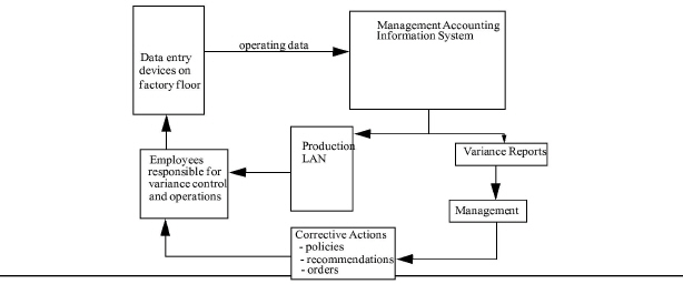
The key objective of variance analysis and reporting is to isolate off-standard performance quickly and correct it. The operational control loop is illustrated in Exhibit 8-1

. Steps necessary to install this opera­tional control loop include the following:

Step 1. Set the standards, prepare the standard cost card, and develop the budgeted manufacturing cost equation. This step was covered in Chapter 7.

Step 2. Collect operating data and measure actual performance. With the use of computers, automated pro­duction equipment, and online data collection and entry devices, measurement may be real-time, whereas in manual-based systems, measurement may be monthly.

Step 3. Process operating data and calculate variances.

Step 4. Report variances to the managers and workers who are responsible for them and have authority to take corrective action. The key for corrective action and operational control is the timely arrival of variance information and immediate action by managers and operating personnel. Variances occur as operations are performed. Therefore, the quicker the variances are reported, the sooner corrective action can be taken, if warranted. For example, if an operation is using excessive amounts of direct materials and the variance indicating this abnormal usage is not reported until a month after the fact, management may not know about the problem and therefore can take no cor­rective action during that month. Cost control must be applied at the place and time where the cost variance originates.

Step 5. Determine the significance of each variance. Some variances require investigation, others do not. In turn, investigation may or may not reveal the need for corrective action.

Step 6. Take appropriate corrective actions. Setting new policies, making recommendations, and giving specific orders to supervisors and workers involved directly in operations are all forms of correc­tive action. Because no set rules or parameters may exist about when to investigate or take correc­tive action, managers and workers often must use their own judgment. A fundamental characteristic of world-class manufacturing is that control (i.e., investigation, problem identifica­tion, and corrective action) occurs on the shop floor as operations are performed. The role of the SCAS as a responsibility accounting system is to capture data on the sources and causes of cost variances and indicate whether corrective actions have been taken. In its daily operational control role, the SCAS reinforces the need for control at the source by requiring input on control activi­ties.

Step 7. Change performance, if possible, to bring actual performance in line with standard performance. Supervisors and workers can change tasks and activities to prevent future variances from occur­ring from the same causes.

Step 8. Revise standards if those previously set are no longer relevant. Standard costs must be revised when prices, rates, operations, product or service specifications, or other circumstances change to such an extent that the existing standards no longer represent a good measure of performance.

Reducing Record-keeping Costs

Information-processing efficiency is increased when record-keeping costs are reduced. Materials requisi­tions and labor time tickets can be prepared in advance of production using the production LAN's bill of materials, MRP and/ or MRP II programs, and the standard quantities from the standard cost cards.

  

In an actual CAS, when a perpetual inventory system is used, the accountant must continuously recalcu­late changing actual unit costs. In a periodic inventory system, RMI costs may be calculated by assuming some inventory flow pattern (FIFO, LIFO, moving average, and so on). In an SCAS, costs can be assigned to WIP, FGI, and COGS accounts based on standard prices and quantities for each cost element. Rather than valuing completed output by performing the cost allocations required in process costing, an SCAS will use the standard absorptive manufacturing cost (SAMC).

   

 

For example, if the SAMC in the printing department of a textbook publisher is $5 per book and the pages for 1,000 books were printed last month, then the journal entry amount transferring printed pages from this department to the binding department would be $5,000 (see Exhibit 6-4 and journal entry 8 in the PCAS). For a JOCAS, if the SAMC for a one-pound box of chocolate-covered cherries is $6.50 and 100 boxes are produced in job 247, then the job's cost is $650.00 for journal entries 8 and 9 (see Exhibit 5-1 and the COGM and COGS journal entries).

Obviously, some of the clerical time and record-keeping costs saved through such simplification is offset by time spent in deriving standards, keeping them current, and calculating and reporting cost variances. The real cost savings occur in the long run, during the implementation of the SCAS when inefficiencies may be identified and corrected and waste uncovered, and later when variances are reported, investigated, and corrected.

Scas Cost Variance Formulas

LEARNING OBJECTIVE 2

Explain the mean­ing of a cost vari­ance, and calculate and interpret the variable costs' spending variances.

Generically speaking, there are only two types of cost Variances: spending (price) variances and efficiency (usage) variances.In this section, the spending variances for the variable manufacturing costs (direct mate­rials, direct labor, and variable overhead) will be illustrated first. Next, the usage variances will be calcu­lated for the variable manufacturing costs, followed by the spending and usage variances for fixed overhead. Finally, alternative methods for calculating overhead variances will be considered. The Nulife Sports Drink Company will be used to illustrate these calculations:

Spending Variances For Variable Costs

The basic formula for a variable cost spending variance is:

Variable cost spending variance = Actual quantity purchased x (Standard price - Actual price)

= AQp x (SP - AP)

DIRECT MATERIALS PRICE VARIANCE. The direct materials standard price is usually based on either the expected price during the period the standard is in effect or on the price existing at the time the standard is set. Normally, this group decision-making activity involves the purchasing department aided by the management accountant.

Many factors influence the price paid for materials, such as quantities purchased, delivery method used, quantity discounts, and rush orders. Serious study should be given to handling and storage procedures to determine whether they are the most efficient possible. Such analysis should indicate the most economical quantities to purchase, the best delivery method at the lowest cost, and the most economical ways of stor­ing and handling in-plant materials.

The direct materials price variance measures the difference between what is paid for a given quantity of materials and what should have been paid according to the standard price that has been set. The formula used to compute this variance is:

Direct materials price variance = AQp x (SP - AP)

In July, Nulife incurred the following price variance for Tigerade's direct materials:

Direct materials price variance

 Explaining the price variance calculation is relatively simple. Forty thousand pounds were purchased at an average price that is $0.10 per pound higher than the standard price. Ten cents per pound multiplied by the 40,000 pounds purchased results in a cost overrun of $4,000-in other words, an unfavorable spending vari­ance of $4,000.¹ While explaining the calculation to shop floor personnel is relatively easy, identifying the cause of the variance may be more difficult.

Generally, the purchasing agent has control over the prices paid for materials and, therefore, is responsible for purchase price variances. This is the first person who should be consulted in attempting to identify the cause of the variance. In Nulife's case, the unfavorable price variance resulted from the pharmaceutical company unexpectedly raising its price $0.10 per pound. The purchasing agent has negotiated a price of $1.05 per pound for the next six months. The new direct materials standard price will be $1.05 per pound next period. In a high-quality SCAS, the explanation for any price variance is recorded on the purchase order. This information is then available as soon as it is known for input into the SCAS database and for use by the MRP II LAN and the marketing LAN in updating sales prices (if possible).

Caution must be exercised to make sure that the purchasing agent is not buying poor-quality material, at a lower cost, to realize a favorable price variance. The poor-quality material will cause problems later in pro­duction. Also, the purchasing agent may increase the purchase order quantity to obtain a lower unit cost. Large inventories, however, require large automated stockrooms and sophisticated inventory tracking sys­tems, which drive up nonvalue-added costs. Maintaining these systems generates even more nonvalue-added activities and costs. Thus, if this purchasing price variance is the only performance evaluation crite­rion for the purchasing agent, he or she may be motivated into these dysfunctional decisions.

In some instances, however, someone other than the purchasing agent may be responsible for a direct materials price variance. The production manager, for example, may schedule production in such a way as to require overnight delivery of materials, thus driving up the price paid for them. The following are sev­eral additional reasons why actual direct materials prices may differ from standard direct materials prices:

• Change of vendor

• Change of lot size

• Change in price by vendor

• Change in specifications

• Change in the marketplace

Two considerations relevant to the design of a high-quality SCAS become obvious. First, the SCAS needs to capture data on the cause of the variance when it first becomes known. Second, once the cause has been identified, its source has to be input into the SCAS so that responsibility can be properly assigned for per­formance evaluation. If the source and cause of cost variances are not captured within the SCAS, then it cannot provide accurate and relevant information for operational control and performance evaluation. In that case, the SCAS may not lead to proper evaluation and rewards and, therefore, may not promote the desired motivations and goal-congruent behaviors for daily control activities.

DIRECT LABOR RATE VARIANCE. The development of a standard direct labor cost requires identi­fying the direct labor classification needed for the operation and the wage rate paid for that labor skill. Rates for labor are often determined by union negotiations or by the prevailing rate in the area where the company is located. The key objective is to match the operations with the labor classifications called for.

The direct labor rate variance measures any deviation from standard in the average hourly rate paid to employees plus the average hourly payroll taxes and fringe benefits paid for them. The formula used to compute this variance for July's production of Tigerade at Nulife is:

Direct labor rate variance

   = Actual DLhr worked x (Standard rate - Actual rate)

   = AQp x (SP - AP)

   = 17,500 DLhr worked x ($10.00/DLhr - $9.50/DLhr)

   = $8,750 favorable

The same basic formula is used for both the direct materials and the direct labor spending variances. The difference between the standard price (rate) and the actual price (rate) is multiplied by the quantity pur­chased. For direct labor, the hours purchased always equal the hours worked because labor is actually “purchased” (paid for) after it is used. Similarly, with a JIT purchasing system, the quantity of materials used and purchased is equal.

As with the direct materials price variance, this variance's calculation is relatively simple to explain. The average labor rate (including the direct labor wage rate plus employer payroll taxes and fringe benefits) was 50 cents per hour less than budgeted. For the 17,500 DLhr actually worked (i.e., for the actual quan­tity purchased), this resulted in a cost savings of $8,750.

In many companies, the rate paid workers is set by union contract. Therefore, in such instances, rate vari­ances tend to be small. The way workers are used can lead to rate variances, however. Skilled employees with high hourly rates of pay can be assigned tasks that require little skill and call for low hourly rates of pay. Such misuse of workers will result in unfavorable direct labor rate variances because the actual hourly rate of pay will exceed the standard rate authorized for the particular task being performed. Also, poor scheduling of work may cause unfavorable rate variances. In addition, workers may have been paid excess rates during peak seasonal periods in order to obtain the necessary work force.

In the Nulife example, just the opposite situation happened during July. The favorable rate variance resulted from hiring part-time help. Total actual labor cost was $166,250. These temporary workers earned a lower hourly wage rate and cost Nulife less in payroll taxes and fringe benefits than the company would have spent if it had used regular workers and paid them overtime. The result was an average savings of 50 cents per hour when the total direct labor costs were averaged over the total hours worked.

VARIABLE OVERHEAD SPENDING VARIANCE. The variable overhead spending variance is the amount budgeted for the number of direct labor hours worked minus the actual VOH costs incurred. This variance is usually the responsibility of the person or persons in charge of such VOH cost items as indirect labor, utilities, maintenance, supplies, and so forth. These costs should be in line with the amount of work performed. For the Nulife case, the VOH spending variance is:

 

 While this “formula” may look different from the formula used for direct materials and labor, it is really the same, just in an unfactored form. To illustrate this, the “actual VOH price” is $1.43 per DLhr (rounded). A price per DLhr must be calculated to compare against the standard price (VOH POR), which is also per DLhr. The quantity used in the formula must then he DLhr as well. Using the basic formula:

VOH spending variance = AQp x (SP - AP)

= 17,500 DLhr worth of VOH items purchased x ($1.501DLhr - $1.43/DLhr)

= $1,225 favorable

The $25.00 difference between these two versions of the formula is due to a rounding error in using the $1.43 average price per DLhr worked. The actual average VOH price per DLhr is $1.42857. Thus, using the unfactored format originally presented avoids this rounding error. The unfactored format can be used for all three variable cost spending variances.² In many SCASs, only the total actual VOH costs may be recorded, not the individual actual prices and rates. In these situations, the unfactored format may be sim­pler and more accurate. With the implementation of an ICBIS, though, fields within computer database records usually exist for storing the unit prices. Also, calculation of unit prices and rates may make the information more usable for the shop floor, where people think in terms of per pound and per hour prices.

The favorable VOH spending variance for Tigerade could have been caused by cost decreases in variable overhead items or the efficient use of these items, or both. To better understand why this is true, consider how the VOH line in the standard cost card is calculated. While total VOH is budgeted by using a DLhr basis, VOH items are not really purchased by the labor hour. Lubricating oil may be purchased in 50-gal­lon drums; drill bits and saw blades by the box of one dozen; and nails, tacks, brackets, and the like in 25-pound boxes. To apply all the VOH items to individual products, they are averaged over the activity basis that causes their use (i.e., direct labor hours for Tigerade). Since the VOH applied is computed by using a standard price (VOH POR) based on direct labor hours, the average actual VOH costs are also averaged over the actual direct labor hours worked to calculate an average VOH price per DLhr for the variance comparison.

Thus, the average actual VOH price per DLhr worked results from the prices of the VOH items purchased and the amount used for the hours actually worked. If the price for certain VOH items is less than budgeted and/or the amount used is less than budgeted for a DLhr, then this variance will be favorable. The variance itself, however, does not provide insight into which factors caused it.

The management accountant should break down the VOH spending variance into the elements comprising it. Exhibit 8-3

illustrates how the variance is presented as a line-by-line analysis. This more complete anal­ysis is much more useful to managers who are responsible for different elements. Although the total VOH spending variance may be small and favorable, such a report is usually necessary. For example, a small favorable VOH spending variance may be the result of large individual favorable and unfavorable over­head item variances offsetting one another.

The second column in Exhibit 8-3 is titled “Flexible Budget for 17,500 DLhr Actually Worked.” A flexi­ble budget is a budget amount calculated using the actual hours worked. It is an “after-the-fact” budget prepared by using the cost equation and the hours actually worked. This is necessary because variable costs exist. Variable costs change in total with changes in production volume and the number of hours worked.

For example, in preparing the original budget for Tigerade, the production quota was 10,000 cases. Using the standard quantity for direct labor (2 DLhr per case), 20,000 DLhr were originally budgeted to be worked, and $30,000 of VOH was budgeted in total (VOH POR of $1.50 per DLhr multiplied by 20,000 DLhr budgeted). The original budgeted $30,000 cannot be compared to the $25,000 actually spent, though, because this amount was spent in working only 17,500 direct labor hours. Of course, if fewer hours are worked, less total VOH should be spent.

For a valid comparison, the budget has to be adjusted to what it should he for the DLhr actually worked. For 17,500 DLhr, only $26,250 in VOH should have been spent (VOH POR of $1.50 per DLhr multiplied by 17,500 actual DLhr worked). This is the “flexible” budget amount that should be compared against the actual VOH costs incurred for the same 17,500 DLhr worked. The spending variance formula automati­cally adjusts for this by comparing (AQp x SP) to actual cost. This can be seen in the unfactored format of the variance formula.

Usage Variances For Variable Costs

As with the variable costs spending variances, there is one basic formula for the variable costs' efficiency variances:

Variable cost usage variance

 The standard quantity allowed (SQA) is the total amount of an input item that should have been used for the actual production volume. The formula for SQA is:

SQA = Standard quantity x Actual output

For example, if one case of Tigerade (in Exhibit 8-2) is made, then:

• SQA Direct materials    = 3 lb. per case x 1 case = 3 lb.

• SQA Direct Labour    = 2 DLhr per case x 1 case = 2 DLhr

• SQA_VOH    = 2 DLhr per case x 1 case = 2 DLhr

If ten cases of Tigerade are made, then:

• SQA Direct materials    = 3 lb. per case x 10 cases = 30 lb.

• SQA Direct labour    = 2 DLhr per case x 10 cases = 20 DLhr

• SQA_VOH    = 2 DLhr per case x 10 cases = 20 DLhr

If 9,000 cases of Tigerade (the actual output) are made, then:

• SQA Direct materials    = 3 lb. per case x 9,000 = 27,000 lb.

• SQA Direct Labour    = 2 DLhr per case x 9,000 = 18,000 DLhr

• SQA VOH    = 2 DLhr per case x 9,000 = 18,000 DLhr

The more cases of Tigerade produced, the more direct materials, direct labor, and VOH items will be used. These are variable costs. The SQA calculation is a flexible budget adjustment for quantities.

In July, 9,000 cases of Tigerade were produced. There were no beginning or ending WIP inventories, or output loss. If partial effort exists in beginning or ending WIP, or in output loss, the partial effort needs to be accounted for by computing equivalent units of production (EUP) for each cost element. This is a stan­dard PCAS. To illustrate, assume an ending WIP inventory in July of 200 cases, 100 percent complete with respect to direct materials, 50 percent complete for direct labor, and 25 percent complete for VOH. The EUPs for July are:

EUP for direct materials    = 9,000 completed cases + (100% x 200 cases)

   = 9,200 EUP

EUP for direct labor    = 9,000 completed cases + (50% x 200 cases)

   = 9,100 EUP

EUP for VOH    = 9,000 completed cases + (25% x 200 cases)

   = 9,050 EUP

Then:

SQA_{Direct materials}    = 3 pounds per case x 9,200 EUP = 27,600 pounds 

SQA _{Direct labour}    = 2 DLhr per case x 9,100 EUP = 18,200 DLhr 

SQA_voh    = 2 DLhr per case x 9,050 EUP = 18,100 DLhr

Throughout the remainder of this chapter, we will continue to ignore the existence of partial effort in beginning WIP, ending WIP, and/or output loss (spoilage). This is to emphasize the concepts and calcula­tions involved in an SCAS. In reality, though, it is important to remember the need for EUP calculations in process system SCASs.

DIRECT MATERIALS USAGE VARIANCE. The direct materials usage variance measures the dif­ference between the actual quantity of materials used in production and the quantity that should have been used (SQA). The formula used to compute this variance is:

Direct materials usage variance = SP x (SQA - AQu)

For the Tigerade example:

Direct materials usage variance    = $1.00/lb. x (27,000 lb. - 30,000 lb.)

   = <$3,000> unfavorable

Like the spending variances, this usage variance is fairly easy to explain. For the 9,000 cases of Tigerade that were produced in July, only 27,000 pounds of direct materials should have been used. But, 30,000 pounds were used. If there is no price variance, then the extra 3,000 pounds used cost Nulife an extra $3,000. This cost overrun is an unfavorable usage variance. But also like the spending variances, the vari­ance by itself does not indicate its underlying cause(s). This information needs to be obtained from the people responsible for direct materials usage.

Generally, the production manager is responsible for the direct materials usage variance because he or she is in charge of how direct materials are used. In instances where direct materials are substandard, the responsibility may lie with the purchasing department. Other causes include the following:

• Incorrect machine settings or lack of proper tools

• Failure to keep machines and tools in good working condition

• Inexperienced or inefficient workers

• Fatigue caused by pressure to complete a rush order

• Changes in production or quality control methods

• Inadequate blueprints or errors in specifications

• Variations in yield from materials

• Failure to return excess materials to the storeroom

In the Tigerade example, the variance was due to inexperienced workers and improper supervision at mix­ing vat 3. A total of 3,000 pounds of compound was spilled on the floor and wasted.

The direct materials standard quantity is affected by the desired size, shape, and quality of the finished product, as well as by the kind and quality of the direct materials used to make the product. An allowance for normal spoilage is included in determining practical standard quantities. The tighter the standard, the smaller the allowance for scrap. When appropriate direct materials standard quantities are in effect, control over material losses, waste, and scrap is facilitated, because any usage variance from what was determined to be a reasonable amount can be traced to its source, as was done in the Tigerade example.

Given the kind and quality of direct materials, physical quantity estimates are made in terms of weight, size, volume, or other measure. The standard quantities and quality of direct materials needed to make the product are compiled in its bill of materials within an MRP or MRP II program. The actual quantities are input via bar code scanning devices, or materials requisitions in nonautomated SCASs.

DIRECT LABOR EFFICIENCY VARIANCE. The direct labor efficiency variance measures the pro­ductivity of direct labor. The basic formula used to compute this variance is the same as that used for the direct materials usage variance:

Direct labor efficiency variance = SP x (SQA - AQu)

During July, the direct labor efficiency variance for Tigerade was:

Direct labor efficiency variance   = $10/DLhr x (18,000 DLhr - 17,500 DLhr)

   = $5,000 favorable

Explaining this variance to shop floor personnel, 500 direct labor hours less than expected (the SQA) were worked. At a budgeted labor rate of $10 per DLhr, this resulted in a cost savings of $5,000 (a favorable usage variance). The Tigerade production manager explained that this efficiency was due to the high spirit of the temporary workers. But remember the cause of the direct materials usage variance--by working so fast, they also wasted 3,000 pounds of Tigerade mix.

This observation provides the management accountant with insights into some of the characteristics required in a high-quality SCAS:

For operational control, it is important that the SCAS captures input data about the sources and causes of cost variances. By having shop floor personnel input these data as operations take place, their attention is focused on the need to identify production problems and control them at the source.

In assigning responsibility for cost variances, these source and cause data are critical. To ensure proper performance evaluation and the rewards necessary for proper employee motivation, the SCAS needs to report the sources and causes of cost variances and whether corrective actions have been taken.

As the Tigerade example shows, one decision (activity) may result in more than one cost variance. In other words, cost variances can be related; they are not necessarily financial measures of independent problems. For July production of Tigerade, the hiring of temporary workers resulted in three cost variances: an unfa­vorable direct materials usage variance of $3,000; a favorable direct labor rate variance of $8,750; and a favorable direct labor efficiency variance of $5,000.

The direct labor efficiency variance is vital for management's review, because increasing productivity in labor-intensive processes is a key to reducing production costs. Generally, this variance is the responsibil­ity of supervisors and workers. In some instances, however, an unfavorable direct labor efficiency vari­ance may stem from areas not controlled by them, such as the following:

• Faulty equipment or materials

• Machine breakdowns

• Lack of materials

• Changes in production processes

Factors that cause the variance to occur can be identified by careful analysis of the operations, which must include discussion with individuals involved in specific areas of the organization. Two important factors used to determine the direct labor standard quantities are:

• Specific operations to be performed

• Amount of labor time to be spent on each operation

Both factors are measured by engineering, production, and management accounting personnel.

Each operation performed by either employees or equipment should be determined. Examples of labor operations are bending, lifting, turning, reaching, moving materials, setting up for a new production run, cleaning up, and reworking. All of these operations will affect the time needed to produce a product. Thus, such operations should be evaluated to determine which are adding value and which can be eliminated or reduced.

Some organizations conduct time and motion studies. During such studies, unusual times due to abnormal conditions should be eliminated. Some industries have developed predetermined times based on standard time and motion studies. Using these data reduces the cost of developing standards for a specific company in one of those industries. Care must be taken, however, to make sure the operations and labor of the com­pany match the operations and labor on which the data were gathered.

Plant layout, equipment conditions, and the workplace should be analyzed, and an effort should be made to improve these to the best practical level (maybe even close to an ideal level). In conjunction with study­ing and setting direct materials and direct labor standards, purchasing and expediting materials should be studied so that employees have the right materials (quality and quantity) at the right place at the right time. Moreover, employees should be properly trained before being put on the job and should have quick access to complete instructions after being put there.

If direct labor standards are based on a work environment that is conducive to maximum efficient and effective operations, variations of actual from standard become valid indicators of what really should be occurring. A poor workplace that is unsuitable for both people and efficient operations will most likely lead to variances whose underlying causes cannot be easily traced.

The direct labor efficiency variance, however, can encourage costly actions by employees. For example, employees may rush through a process wasting costly materials to improve labor efficiency as happened at Nulife during July.

The direct labor efficiency variance may have little relevance in a highly automated plant that has few employees. For example, some companies, such as Allen-Bradley, manufacture over $100 million worth of products per year and employ only three to five workers.

VARIABLE OVERHEAD EFFICIENCY VARIANCE. The variable overhead efficiency variance is a measure of the excess VOH used solely because the actual direct labor hours worked differed from the standard hours allowed. Tie assumption is that if more direct labor hours are worked, then more VOH items are used (VOH is a variable cost). This variance can be computed using the following formula (the same basic formula used with the direct materials and labor efficiency variances):

VOH efficiency variance = SP x (SQA - AQu)

During July, the VOH efficiency variance for Tigerade production was:

VOH efficiency variance    = $1.501DLhr x (18,000 DLhr - 17,500 DLhr)

   = $750 favorable

The assumption that more labor usage means more VOH items are used is questionable. For example, the temporary workers at Nulife in July wasted 3,000 pounds of Tigerade mix by working too fast. Did they also use excess VOH items such as supplies? The VOH efficiency variance does not really answer this question, but from looking at the VOH spending variance, it appears that excess usage of indirect items was not a problem. Again, this highlights the major disadvantage of traditional cost variance analysis. Variances alone do not provide information about their real underlying causes.

Whether favorable or unfavorable, the responsibility for this variance lies with the manager in charge of labor for the period (if labor causes VOH usage). Other bases, such as machine hours, can also be used to budget VOH and measure its variances.

Fixed Overhead Cost Variances

LEARNING OBJECTIVE 4

Calculate and inter­pret the fixed over­head variances.

With each of the variable cost elements, there are fundamentally only two kinds of cost variances, spend­ing and usage. This is also true for fixed overhead, but the formulas for the FOH cost variances differ from the variable cost variances because this cost element behaves differently. It is a fixed cost, not a variable cost.

FIXED OVERHEAD BUDGET VARIANCE. The fixed overhead budget variance is the difference between budgeted fixed overhead costs and actual fixed overhead costs:

Fixed overhead budget variance = Budgeted FOH - Actual FOH

In the Nulife Tigerade example, the following FOH budget variance resulted in July:

Fixed overhead budget variance = $12,000 - $12,100 = <$100> unfavorable

During July, $100 more was spent on FOH items than was budgeted ($12,000 from its manufacturing cost equation in Exhibit 8-2). The unfavorable FOH spending (budget) variance is the responsibility of the vari­ous people who have control over the different items that comprise the total budgeted FOH costs. Gener­ally, managers have only limited ability to control FOH costs in the short run, however. Fixed overhead costs are incurred to provide production capacity. In other words, FOH exists because of the production process (the factory) and its size. The bigger the factory, the larger its fixed costs (usually), such as build­ing depreciation, insurance, property taxes, and the costs of heating and air conditioning. Because different people are responsible for different components of FOH, the SCAS should report this variance on a line-item basis, similar to the reporting of the VOH spending variance (see Exhibit 8-3). Exhibit 8-4

illustrates a line-by-line FOH budget variance report.

Any control that is to be exerted over FOH must take place when managers are preparing the annual bud­get, modifying it during the year, and/ or planning capacity changes. Fixed overhead items, therefore, are usually not subject to as much day-to-day, or even month-to-month, control as are variable cost items.

FIXED OVERHEAD PRODUCTION VOLUME VARIANCE. This variance is usually called the fixed overhead volume variance, or just the volume variance. It is a usage variance in that it measures how well the factory as a whole was used. Since the costs of the factory are FOH costs, this is an FOH usage variance. It can be calculated by either of two formulas:³

FOH volume variance

   = FOH standard cost x (Actual output - Production quota)

or:

   = FOH standard price x (SQA - Budgeted DLhr)

The second formula more closely resembles the formula for variable cost usage variances and may be eas­ier to learn because of its similarity to the other usage variance formulas. First, the basis for applying FOH has to be known. This information is in the standard cost card (Exhibit 8-2 for Tigerade). Fixed overhead is applied to cases of Tigerade based on the DLhr worked. Thus, the standard hours allowed (SQA) and the budgeted DLhr need to be calculated in order to use this version of the volume variance formula. The budgeted DLhr for July were 20, 000.⁴ Using DLhr and the FOH POR in this formula:

FOH volume variance    = $0.60/DLhr x (18,000 DLhr - 20,000 DLhr)

   = <$1,200> unfavorable

If the FOH POR (standard price for FOH) is based on machine hours, then the standard machine hours allowed and the budgeted machine hours would be used.

The first version of this variance formula may be easier to explain, however. To illustrate, the FOH vol­ume variance for Tigerade is calculated as:

FOH volume variance    = $1.20/case x (9,000 cases - 10,000 cases)

   = <$1,200> unfavorable

The FOH volume variance measures how efficiently the entire plant is used. Using the output-based for­mula, 10,000 cases of Tigerade were budgeted for July production. The FOH cost budgeted was $12,000 (reference the cost equation in Exhibit 8-2). Thus, only $1.20 of FOH cost had to be absorbed by each case (this is the FOH standard cost). In other words, if the sales price is increased by $1.20 per case, and 10,000 cases are produced and sold, Nulife will receive extra sales revenues of $12,000 that can be used to pay for the FOH. One of the benefits of a standard absorptive manufacturing cost is that it serves as an aid to ade­quate sales price setting.⁵

In July, however, Nulife produced only 9,000 cases of Tigerade, not the 10,000 planned for. Thus, there were 1,000 cases not produced and not sold. Because these cases were not sold, Nulife cannot recover the extra $1.20 from each needed to pay for the FOH costs. The 1,000 cases not produced, multiplied by the $1.20 FOH standard cost, equals $1,200 (10 percent of the $12,000 budgeted FOH). This $1,200 of sales revenues is needed to pay for the last $1,200 of FOH costs. Since the revenues are not there, the remainder of the FOH will have to he paid for out of the profits made on the 9,000 cases produced and sold. Total profits will be $1,200 less than they should have been for the 9,000 cases sold, because the production quota was not met. Because the plant was not used as efficiently as planned, profits went down. This is equivalent to the lower profits that result from inefficient use of labor or materials (their usage variances). The plant is just another manufacturing resource, like materials and labor, and using it inefficiently creates a usage variance just like the other manufacturing inputs.

The usefulness and interpretation of the FOH volume variance depend on the volume used in calculating the FOH standard cost. In the Nulife situation, expected capacity was used. Nulife could have used normal, practical, or theoretical capacity (refer back to Exhibit 7-9). If any of these three options had been chosen, the usefulness and interpretation of the FOH volume variance would have been different.

For example, WCM proponents might use theoretical capacity in determining the FOH standard cost. The difference between this maximum productive capacity and the actual output measures how much of the plant is idle. While this may be by design, a continuous improvement philosophy means that the volume variance should get smaller over the years. Here is yet another example of how a high-quality SCAS should report long-run trends in variances.

When expected capacity is used to set the FOH standard cost, an unfavorable volume variance is due to lower than budgeted production. This is often caused by a lack of sales orders. Lack of sales orders may be caused by one or a combination of the following:

• High prices for the product

• Low quality of the product

• Inadequate advertising and lack of aggressive sales campaigns

• Inability to deliver when customers want the product

• Economic recession

Some other causes of unfavorable volume variances are controllable by plant management:

• Poor job scheduling

• Excessive employee absenteeism

• Shortage of direct materials and supplies due to poor planning

• Breakdown of machines due to poor preventive maintenance

• Inadequate training or supervision of workers

COMBINING THE OVERHEAD VARIANCES. In the preceding discussions, two variances (spending and usage) were calculated for each cost element (direct materials, direct labor, VOH, and FOH). Note that for overhead, spending and usage variances were separately calculated for VOH and FOH, resulting in a total of four overhead cost variances. These were separately calculated because the variances are con­trolled by different people (responsibility centers).

In traditional CAS designs, though, VOH and FOH were not separately accounted for. In Chapters 4, 5, and 6, VOH and FOH were combined into just one total overhead (TOH) account, and only one TOH POR was used to apply overhead to products. Unless VOH and FOH are separated in the SCAS, calculating four overhead variances is difficult.

Consequently, in many traditional SCASs, fewer than four overhead variances were prepared for manage­ment. Presenting all four overhead variances is called “four-way analysis of overhead.” Sometimes only three overhead variances are calculated (“three-way” analysis), or only two variances (“two-way” analy­sis), or just one TOH cost variance (“one-way” analysis).

These simpler presentations result in less useful information and degrade the quality of the SCAS. Never­theless, these methods still often appear on professional accounting certification exams (CPA, CMA, CIA), so they will be briefly illustrated here. There are two “tricks” to remember in performing three-way, two-way, or one-way overhead analysis. First, four overhead variances have already been calculated. In three-way analysis, two variances are added together. In two-way analysis, three of the four overhead vari­ances are added together. In one-way analysis, all four overhead variances are added together.

The second “trick” is to know which variances to calculate first. This involves two steps. The first vari­ance to calculate is the total overhead variance. This is the sum of the four variances and represents the one-way method. The total overhead variance is the difference between the TOH applied to production and the TOH actually incurred:⁶

For Tigerade,

TOH applied = TOH POR x SQA

TOH applied = $2.10/DLhr x 18,000 DLhr = $37,800

The actual TOH in July equalled $37,100 (VOH of $25,000 plus FOH of $12,100 as shown in Exhibit 8-2). The difference is $700 favorable. This can be verified by adding together the four overhead cost vari­ances:

VOH spending variance    = $1,250 favorable

VOH efficiency variance    = $750 favorable

FOH budget variance    = < 100> unfavorable

FOH volume variance    = <1,200> unfavorable

TOH variance    = $ 700 favorable

The second variance to calculate is the FOH volume variance. This variance is one of the cost variances in two-way, three-way, and four-way analysis. Knowing the TOH variance and the FOH volume variance, two- and three-way analysis can be quickly performed.

In two-way analysis, the two variances are the FOH volume variance and the “everything else” variance. This is simply the difference between the TOH variance and the FOR volume variance and is often labelled the “TOH budget variance”:

TOH variance    = $ 700 favorable

Less FOH volume variance    = < 1,200> unfavorable

TOH budget variance    = $1,900 favorable

This is also the sum of “everything else” (VOH spending and efficiency, and FOH budget variances).

To prepare three-way analysis, calculate the VOH efficiency variance. The three cost variances arc the FOH volume variance, the VOH efficiency variance, and “everything else” (the sum of the VOH spending and FOH budget variances, which is often called the TOH spending variance).

Summary Of Cost Variance Formulas

Cost variance analysis is really not as difficult as it may seem at this moment. There are only two types of cost variances, spending and usage. There are four kinds of manufacturing inputs: direct materials, direct labor, variable overhead, and fixed overhead. Since each has its own spending and usage variance, there are eight cost variances in total. All of the variable costs, though, use the same formula for their spending variances. They also use the same formula for their usage variances. The fixed overhead variances' formu­las are a little different. The formulas are summarized in Exhibit 8-5.

 

The cost variances also can be combined into. a general model approach to cost variance analysis. This is accomplished by grouping the direct materials variances together, then the direct labor, VOH, and FOB variances. The general model also includes the total cost variance for each input. Exhibit 8-6 presents this general model approach for Nulife's Tigerade variances for direct materials and direct labor during July.

  

 

 Exhibit 8-7 illustrates the variable and fixed overhead cost variances for Tigerade.

Scas Journal Entries

LEARNING OBJECTIVE 5

.Prepare the jour­nal entries for an SCAS, and the cost variance report.

SCASs can be used in job order, process, and JIT systems. Jobs, departments, or cells (in a JIT) are deb­ited with the costs of the manufacturing inputs used. The journal entries in an SCAS, versus a normal JOCAS or PCAS, differ in two basic ways, however:

First, in an SCAS, the cost amounts used are not the same as in a PCAS or JOCAS. Instead of recording actual costs, all cost elements are recorded at standard cost allowed (SCA). SCA is the standard cost for each input multiplied, by production volume. To demonstrate, the standard cost for direct materials in Tig­erade (Exhibit 8-2) is $3 per case. If 10 cases are produced, the SCA is $30 for direct materials, and this is all that will be charged to its cost for direct materials. For production of 10 cases, the direct labor SCA is $200. The VOH and FOH SCAs for 10 cases are $30 and $12, respectively. Either of two formulas can be used to calculate SCA:⁷

SCA    = Standard cost x Actual output

   = Standard price x Standard quantity allowed (SQA)

In an SCAS, the total production cost assigned to 10 cases of Tigerade is $272. This is calculated by sim­ply summing the SCA for each input item or by the following formula:

Total production cost    = SAMC x Actual production volume

   = $27.20/ case x 10 cases

   = $272.00

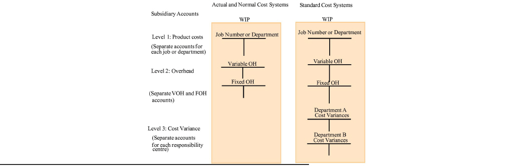
The second difference between normal and SCAS journal entries is related to the first. Since all inputs, and production volume in total, are costed at standard, then the difference between SCA and actual cost also is journalized.

In other words, each cost variance is journalized into its own subsidiary y account. Actual and normal cost systems have two “levels” of general ledger subsidiary accounts, product costs and overhead. SCASs have three “levels” of subsidiary accounts. This is highlighted in Exhibit 8-8

.

In Exhibit 8-8separate VOH and FOH subsidiary WIP accounts are created, consistent with the discussion of separately budgeting for each of these cost elements in Chapter 7. Chapter 7 also pointed out the need to assign cost variances to responsibility centers for proper performance evaluation. This is illustrated in Exhibit 8-8 by having two production departments (A and B), each with its own subsidiary cost variance account. This exhibit should be compared to Exhibits 4-2 (basic CAS), 5-1 (JOCAS), and 6-4 (PCAS).

Standard Pcas Journal Entries

In Chapter 4, three basic types of journal entries were identified:

• Purchasing inputs (materials, labor, and overhead)

• Using inputs in manufacturing (materials requisitions, labor distribution, and overhead applications)

• Transferring completed production (between departments in a PCAS, to FGI for COGM, and to COGS when sold)

PURCHASING MANUFACTURING INPUTS. Journal entry 1 records the purchase of raw materials. In the SCAS for Nulife (Exhibit 8-2), the journal entry to record the purchase of Tigerade drink mix (its direct material) is:

 

Tigerade mix, being a special direct material, has its own subsidiary ledger account within RMI. The price variance is recorded when the materials that create it are received.

An unfavorable cost variance is debited to the cost variance account. An unfavorable cost variance is a cost overrun. Paying for this increased cost reduces (credits) cash. If cash is credited, then the cost vari­ance account must be debited. Conversely, a favorable cost variance is a credit amount within the journal entries. Favorable variances are cost savings. Saving costs increases (debits) cash. Thus, the cost variance account is credited.

The information explaining the variance should be available from the purchase order for entry into the SCAS. If a record field is established for the explanation, or a general ledger coding system is created to identify its cause, then the cause can be input and reported. The ability to capture and report information on the causes of cost variances is a characteristic of a high-quality SCAS.

Journal entries 2 and 3 recording payroll and the employer's related liabilities are the same in all CASs. In recording actual overhead costs (journal entry 4), separate WIP subsidiary accounts are created for VOH and FOH. Assume that the $25,000 in actual VOH costs (Exhibit 8-2) represents utilities costs for July that are paid for in cash and that the $12,100 of FOH represents July's factory depreciation. Journal entry 4 to record these costs is:

 

USING MANUFACTURING INPUTS IN PRODUCTION. Journal entries 5-7

record the issuance of materials, labor, and the application of overhead to production departments. When the journal entries for assigning these costs were made in a normal PCAS, each department was charged with the materials and labor costs directly traced to it and with the overhead applied to it. This resulted in multiple subsidiary accounts (one for each department) being debited in journal entries 5-7.

In a process costing SCAS, though, each department's usage is journalized separately. To illustrate, instead of having one journal entry 5 for direct materials used in Departments A and B, a separate journal entry is made just for Department A's usage. Another journal entry is made to record direct materials usage in Department B. Preparing individual journal entries for each department's usage of direct materials, direct labor, and applied overhead facilitates the recording and control of each department's cost variances. To demonstrate using the Tigerade example, assume that the costs shown in Exhibit 8-2 are only for Depart­ment A:

 

Because the price variance was already recorded in journal entry 1 when the direct materials were pur­chased, materials enter RMI at their standard price. Thus, when these materials are requisitioned into the production department, they are taken out of (credited to) RMI at standard price.

Notice that the usage of direct labor and overhead are recorded by a different method. These were journal­ized (debited) into their “temporary holding accounts” at their actual costs. When these inputs are used in production, they arc removed (credited) from their holding accounts at actual cost. The SCA is debited to WIP (as was done above for direct materials), and both the spending and usage variances are recorded in journal entries 6 and 7:

   

   

In the above journal entries, each Department A cost variance has its own subsidiary account. When this is compared to Exhibit 8-8, it is clear that the Exhibit 8-8 cost variance accounts for Departments A and B are actually control accounts. The reason for having individual subsidiary accounts for each department's cost variances is that some of the variances may not be the responsibility of the department's manager. By hav­ing separate variance accounts in the general ledger system, the account balances can be reported to the responsibility center that really caused each variance.

JOURNAL ENTRIES FOR COMPLETED PRODUCTION. The production costs have been debited to the department's subsidiary ledger account at SCA. Thus, when output is transferred to the next depart­ment or to FGI, and then to COGS, SCA is the amount to use in journal entries 8-10:⁸ 

 

To demonstrate the transfer of finished goods from the factory to finished goods inventory, assume that Tigerade is moved from Department A to FGI:

 

Finally, the journal entry to record COGS is:

Standard Jocas Journal Entries

Traditionally, SCASs have been used more in PCASs than in JOCASs. However, the need for effective and efficient cost management is just as crucial in job order systems as it is in process systems. This was first demonstrated in Chapter 5 in the illustration of construction cost budgeting and control (Exhibits 5-21 and 5-22).

In job order enterprises (e.g., construction, print shops), in for-profit services (CPAs, engineers, and law­yers), and in certain merchandising firms (such as distribution centers), the need for cost control is fast becoming a serious management concern. This is also true in nonprofit services, such as hospitals and government services. With increasing public and national concern over health care cost management, the role of the modern management accountant is becoming more important. Standard costing and cost vari­ance analysis can have a significant impact on cost management in the economy's service sector.

Whether cost variances are journalized within the SCAS or just calculated and reported within a normal JOCAS, information about them is essential for proper cost management. One advantage of journalizing cost variances is that the subsidiary accounts provide the basis for reporting this information. The cost variances are isolated within separate accounts, and a formal record exists within the SCAS for both short-run cost variance reports and long-run trend analyses.

In designing the general ledger system for WIP, level 1 subsidiary accounts are established by department in a PCAS and by job in a JOCAS. This only creates a difference in journal entries 5-7 representing the use of manufacturing cost elements in production. Continuing the Tigerade example, assume the 9,000 cases produced in July was just one job order (482) and that there are still two production departments. As with the PCAS journal entries above, the costs incurred in Exhibit 8-2 are for Department A. In a standard JOCAS, these journal entries become:

   

    

   

    

             

The amounts calculated are the same as in a standard PCAS. There are only two differences in the general ledger account titles;

• The WIP subsidiary accounts for product costs are organized by jobs instead of by departments.

• The department cost variance accounts have posting references for cost variances caused within specific jobs.

Why are posting references needed for the cost variance subsidiary accounts? Consider the dilemma faced by the Department A manager. His department worked on seven different jobs during the month, and his direct labor usage variances stemmed from a number of different sources and causes. To understand which jobs created which labor usage variances, the manager needs to know cost variance information by job. A high-quality SCAS has to capture this information. This is the role of the posting references for jobs. Through a screen display or a hard-copy report, the Department A Direct Labor Efficiency Variance account can provide this information. An example of a departmental report for direct materials usage vari­ances by job is presented in Exhibit 8-9.

Some cost variances, however, may not be directly traceable to specific jobs. If a job does not have any unique (direct) fixed overhead costs budgeted for it, the FOH budget variance may only apply to the month's activities of the department as a whole. Thus, the FOH budget variance would be calculated monthly for the department, as in a standard PCAS. Similarly, the FOH volume variance may or may not be attributable to individual jobs. It may also have to be calculated for the department as a whole on a monthly basis. JOCAS and PCAS SCAS journal entries are compared in Exhibit 8-10.

Disposition Of Variance Account Balances

The balances in the subsidiary ledger cost variance accounts can be disposed of in one of three ways:

• Transferred with the products to FGI and/or COGS

• Closed to the cost of goods sold account at year-end

• Closed to COGS, FGI, and WIP accounts at year-end

As jobs or processes are completed, the variances created by this work theoretically can be transferred with the completed output to FGI and then to COGS.

This has the effect of establishing an actual cost system. If the balances are insignificant, they can be closed to COGS as jobs are sold or at the end of each reporting period for interim financial statement preparation.

On the other hand, the balances can be left in these subsidiary accounts until year-end. Then, these account balances can be disposed of in the same manner as an ending over- or underapplied overhead balance is disposed of in a normal CAS.⁹ If they are significant, they should be pro-rated between the year-end bal­ances in WIP, FGI, and COGS. If they are insignificant, they can be written off directly to COGS.

When overhead is applied to products (jobs or departments), the total actual overhead costs are credited to the VOH and FOH subsidiary accounts.¹⁰ The difference between the overhead applied and the actual overhead costs is journalized to four overhead cost variance accounts. In a normal CAS, this difference is not journalized to special cost variance accounts. Instead, it remains in the overhead account. in other words, over- and underapplied overhead is the sum of the four overhead cost variances. Therefore, it is consistent to treat the disposition of cost variance account balances in the same manner as the ending over­head account balance in a normal CAS.

Reporting Cost Variances

A high-quality SCAS possesses the following characteristics:

Information is timely. For operational control, cost variance information needs to be available in a real-time mode.

Relevant information is reported. For operational control, the SCAS needs to capture information on the real sources and causes of cost variances and on whether the problems causing them have been corrected. For performance evaluation, cost variances need to be assigned to the responsibility centers where they were created.

The reports and screen displays need to present information in a usable format. The SCAS should present information in a manner consistent with the way its users think about it. The SCAS should also help users assess the significance of the cost variances.

Multi-user Report Format

In world-class enterprises with computerized SCASs, multiple reporting formats can be designed to satisfy these needs. In simpler environments, however, a management accountant may have to make do with access to spreadsheet programs. This is the situation Rod Sterling, the management accountant found' him­self in at Nulife. Realizing that the cost variance information had multiple users, he prepared the spread­sheet program shown in Exhibits 8-11 and 8-12.

 

 

 

Exhibit 8-11 contains the top half of the program. This information includes a data section for both the standard costs and actual costs and quantities used in making Tigerade during July. It also includes the standard cost card and manufacturing cost equation. Exhibit 8-12 contains the report that Rod Sterling believes is most useful to shop floor personnel, upper management, and financial accounting for journal entry preparation.¹¹

Rod includes the data sections and standard cost card information in the copies sent to both the shop floor personnel and upper management. This is to alert them to the normal input loss budgeted in the practical standards. A 10 percent normal spoilage rate is allowed for direct materials. Although only 2.7 pounds of Tigerade mix are actually needed to make a case, 3.0 pounds are allowed for input (the standard quantity). The normal spoilage costs Nulife $0.30 per case. There is also a 10 percent loss of labor time. Only 1.8 DLhr of productive time are needed to make a case of Tigerade, but the standard quantity is 2.0 DLhr because of breaks, setup time, and cleanup time. Nulife shop floor personnel have worked hard to reduce setup time to a minimum. Even though the 10 percent labor time lost costs Nulife $2 per case, manage­ment does not believe any additional efficiencies could be realized. To reduce standard labor cost, the pro­ductive time required will have to be reduced (e.g., through learning or production process redesign).

The report shown in Exhibit 8-12 is sent to multiple users. Upper management wants to know the effects of the cost variances on profits. Therefore, Rod Sterling includes a total costs column. In total, profits from July Tigerade production and sales are $7,450 above budget (a net favorable total cost variance). Although the shop floor is excited about this, upper management is not. This favorable variance is only $0.83 per case and only 3.04 percent of SCA. Upper management is more interested in the number of sig­nificant individual cost variances and whether these problems are now under control.

The shop floor personnel are more interested in the per unit column information, because this is how they usually think about production activities. For example, the purchasing agent is worried about the $0.10 per pound direct materials price variance as it is 10 percent over the standard price.¹² Similarly, the shop floor is concerned about the direct materials usage variance and the FOH volume variance. The direct labor usage variance was 0.33 lbs. per case (11.11 percent over the 3 lb. per case SQ). The FOH volume variance averaged $0.13 per case ($1,200 / 9,000 cases actually produced; $1,200 / $12,000 = 10 percent over bud­get). Both, however, were caused by the temporary employees and are not expected to recur again in August. The shop floor personnel are worried that the favorable direct labor variances may not occur again. These were also caused by the temporary help. Their concern is justified because without the favor­able direct labor variances, the total cost variance for July would have been unfavorable.

In reviewing the total costs column, the shop floor was excited over the large favorable direct labor vari­ances, as many people might be over an extra $8,750 and $5,000 in profits. Upper management was not overly impressed, however, and reminded the shop floor personnel that looking at the absolute dollar value of a cost variance can be misleading. From Nulife's point of view, as a multi-million dollar operation, nei­ther the $8,750 nor the $5,000 was significant, representing variances over standard of only 5 percent and 2.78 percent, respectively.¹³

Rod Sterling, though, was proud. He recognized that:

• Shop floor personnel often think on a per unit basis, and he provided this information to them.

• Upper management wanted information on the total costs and effect of the variances on total profits. The report also contained this information.

• Both users need information on the significance of the cost variances, and the percentage of standard cost column provides that information to help them keep a proper perspective.

Finally, Rod thought that the last column noting which general ledger accounts should be debited and cred­ited provided useful information to general ledger accounting personnel. All they have to do is “pull” the total costs from the report for each account. Each of the amounts in the total costs column should be veri­fied by referring back to the journal entries presented in the previous section on standard PCAS journal entries. This last column was only included on the copy printed for financial accounting.

The controller wanted an explanation of how Rod Sterling calculated the total actual costs shown in the cost variance totals section at the bottom of the report. The total actual costs of $237,350 includes five amounts:

• Actual direct labor costs of $166,250

• Actual VOH costs of $25,000

• Actual FOH costs of $12,100

• Actual direct materials used multiplied by its standard price (30,000 lb. x $1.00/lb. = $30,000)

• Plus or minus the direct materials price variance. A favorable variance is subtracted as it represents a cost savings. An unfavorable variance is added. Thus, the $4,000 unfavorable variance is added to the total actual costs.

Celebrating his perceived success that Friday night at the local pub, Rod ran into an old college friend, Linda Onestepahead. Linda earned a masters degree in management accounting and was now CFO of Eaton Corporation.¹⁴ After a few moments of discussing their relative successes, Rod was no longer so proud of himself. He realized that he still had a great deal to do if Nulife's SCAS was to be transformed into a high-quality responsibility accounting system. Not wanting to wait until Monday morning, he excused himself, went home, and began working on an entity relationship diagram (see Chapter 3) and technology platform for a new ICBIS.

Accounting For Loss

One suggestion Linda made to Rod could be immediately incorporated into the cost variance report. At Eaton, she reports nine cost variances for each department. The additional cost variance is for total output loss (normal and abnormal spoilage) consistent with the presentations of world-class accounting for spoil­age in Chapters 5 and 6.

Rod realized that no additional changes are needed to account for input loss. Normal input loss is accounted for within the standard quantities for direct materials (scrap) and direct labor (downtime). Abnormal input loss equals the direct materials, direct labor, and variable overhead usage variances.

Production Mix And Yield Variances

In the Nulife case, only one type of direct material and one class of direct labor were involved in the pro­duction of Tigerade. Many enterprises, however, use a combination of several direct materials and various classifications of direct labor to manufacture products. When a company uses more than one direct mate­rial in its product, one goal is to combine the materials in such a way as to produce the desired product quality in the most economical manner. Some direct materials can be substituted for others without affect­ing product quality.

Direct labor, in some instances, can also be combined in many different ways to produce the same product. Some combinations will be more expensive than others, and some will be less expensive. In situations like this, the direct materials usage variances are related, as are the direct labor efficiency variances. One type of material may have a favorable variance, while another has an unfavorable variance because of substitut­ing one for the other. To better understand the net total usage variance from substitutions, the usage vari­ances for direct materials, as well as for direct labor, need to be combined and reorganized into two summary variances:

• Mix variance

• Yield variance

The Mylantic Chemical Company case on the following page illustrates the direct materials and direct labor mix and yield variances. These variances will be calculated for Mylantic's “cash cow” product, which is Alphachem.

Direct Materials Mix And Yield Variances

The direct materials mix variance results when direct materials are mixed in a ratio different from the standard direct materials formula. The direct materials yield variance is the result of obtaining an output different from the one expected based on the total quantities of direct materials placed in process. Together, these variances make up the direct materials usage variance.

  

During the past week, 120,000 pounds of materials (composed of 46,000 pounds of X, 44,000 pounds of Y, and 30,000 pounds of Z) were placed in process. Nine hundred bags of Alphachem were produced. A total of 3,800 direct labor hours were worked (composed of 950 of A and 2,850 of B).

Exhibit 8-13

presents the calculations of the direct materials mix and yield variances.

The direct materials mix variance is similar to a spending variance in that it measures how much money is saved (or extra money spent) by changing the mix of direct materials. Less than the expected amount of Y and too much x and Z were actually mixed together in the process. Because x and Z are cheaper per pound than Y, the resulting average standard price from changing the mix creates a favorable variance of $18,000.

The direct materials yield variance is the combined usage variance that results from changing the mix ratios, in other words, from inputting the actual quantities of each direct material. Inputting 120,000 pounds in total should have yielded more output than 900 bags of Alphachem. Only 112,500 pounds should have been input for this actual production volume.

The total direct materials mix variance of $18,000 favorable plus the total direct materials yield variance of $45,000 unfavorable equals the total direct materials usage variance of $27,000 unfavorable for all three materials. The trade-off of materials (changing the mix) cost Mylantic $27,000.

Direct Labor Mix And Yield Variances

The direct labor mix variance shows the change in the average standard labor rate from changing the combination of higher- and lower-paid workers. The direct labor yield variance presents the results of using more or fewer total direct labor hours than the standard allowed. The sum of these variances equals the direct labor efficiency variance. Exhibit 8-14 presents the calculations of Mylantic's direct labor mix and yield variances.

As far as the unfavorable direct labor mix variance of $760 is concerned, Mylantic spent an extra $760 by using the actual mix of direct labor rather than the standard. A greater proportion of more expensive labor (Class A) than specified in the standard mix was used. The standard mix is 20 percent of Class A and 80 percent of Class B (1 hour of A and 4 hours of B). The actual mix of direct labor used was 25 percent of Class A and 75 percent of Class B. This drove up the average standard labor rate to $7.00, producing this unfavorable labor spending variance.

In spite of substituting a greater proportion of Class A labor than required at standard, a favorable direct labor yield variance of $4,760 occurred. The total actual direct labor hours of 3,800 were less than the total 4,500 standard direct labor hours allowed for the actual output produced. By working more type A labor hours, fewer type B labor hours were needed, creating this favorable net usage variance. The total direct labor mix variance of $760 unfavorable plus the total direct labor yield variance of $4,760 favorable results in a total direct labor efficiency variance of $4,000 favorable.  

 

Standard Cost Accounting Systems In Jit Processes

LEARNING OBJECTIVE 6

Design a high-qual­ity SCAS with management reports useful for operational control and performance evaluation.

With the advent of world-class manufacturing and JTT conversions, many modern management accoun­tants are rethinking the design of SCASs. Should the SCAS be designed as a process, job order, or hybrid cost system? In part, this depends on:

• The products' cycle times (lead times)

• The information needs of the shop floor personnel and how they want cost variance information dis­played

• The sophistication of the information system

For example, since products are made one-at-a-time in a JIT, the management accountant may want to track input costs to each one, as if it were a job. This makes sense only if the product has a relatively long production lead time. If product production lead times are relatively short, however, treating production cells as departments (or processes) and tracking input costs to them within a PCAS design may be more appropriate. Even though products are pulled through the cells one-at-a-time, tracking costs to each prod­uct, as in a JOCAS, may not be feasible.

In considering shop floor information needs, production workers may only want variance information expressed in quantities, such as the “Per Unit” column information in Exhibit 8-12's report. When a JIT philosophy of continuous improvement is employed, all variances are considered significant, war

rating special attention. Thus, there is no need to convert a direct materials or direct labor usage variance from pounds per unit, or hours per unit, into dollars or percentages of standard. In such situations, journal­izing cost variances may not be a value-added activity. A simpler SCAS can be used, such as a backflush CAS discussed below.

Before deciding what type of SCAS to use, the sophistication of the total information system must be con­sidered. if the enterprise has a highly automated production process with a sophisticated ICBIS, bar cod­ing and reading on the shop floor, and a visual factory, then variance information is available within a real-time mode.¹⁵ The SCAS may not add any new information that is useful in daily operational control activi­ties.

In contrast, if there is no other production control system, then the SCAS may have to calculate, journalize, and report cost variance information. A simple SCAS, such as a backflush system, may not provide the information needed for operational control. At the other end of the SCAS design continuum is a sophisti­cated SCAS that can report cost variances by production activities within each JIT cell. This SCAS will also be illustrated below.

The modern management accountant cannot design an SCAS in isolation from the other information sub­systems within the enterprise. Whatever SCAS is chosen must be congruent with the information needs of the firm, the other information gathering and reporting systems (e.g., MRP or MRP 11, EDI, visual fac­tory), the technology platform available, and the reward systems used. Simpler SCASs are not always bet­ter SCASs. The challenge facing the modern management accountant is to look beyond the SCAS to the whole information system. “Does the entire information system satisfy the needs of the enterprise?” is the question that the management accountant must ask and answer.

Backflush Cost Accounting System

All the cost systems previously developed, from the basic CAS in Chapter 4 through the standard PCAS and JOCAS in this chapter, track input costs throughout the production process. A backflush cost accounting system (BCAS) does not. There is no WIP account within this system's general ledger. WIP is replaced with a raw-in-process (RIP) general ledger account. RIP, however, includes only the raw materi­als purchased. Direct labor and overhead costs are journalized into a “Conversion Costs” account. Costs are not taken out of these accounts until the product is completed (the COGM journal entry 8 in a JOCAS, or 9 in a PCAS). In this way, costs are “flushed out of the general ledger” when production is completed.¹⁶ Exhibit 8-15

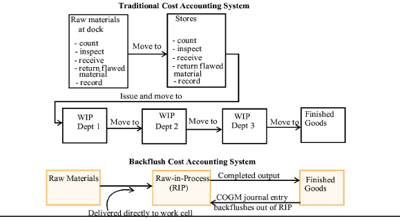
 illustrates the basic differences between a traditional PCAS and a JIT using a BCAS. A BCAS differs from the more traditional systems in four ways:

• Raw materials are debited to RIP instead of RMI.

• Direct labor and overhead are debited to Conversion Costs (DL + OH) instead of Gross Wages and WIP-Overhead.

• No input usage journal entries are made as production takes place. The use of materials, labor, and over­head is recorded “after-the-fact” in the COGM journal entry.

• Cost variances are not journalized in the BCAS.

July's COGM journal entry for Tigerade production at Nulite using a BCAS becomes:

 

Exhibit 8-16

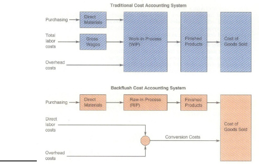
 contrasts the cost data flows for a traditional PCAS and a BCAS where no FGI is maintained in a JIT. Here, the “trigger point” for recording input usage is the COGS journal entry. COGS, instead of FGI, is debited at SCA.

FOCUSING ON OUTPUT. A BCAS focuses first on the output of an organization and then works back­ward when assigning costs to FGI or units sold. The term “backflush” comes from the technique of delay­ing journal entries until products are completed (or as late as sales in some BCASs), when costs finally are flushed through the accounting system. This approach is opposite to traditional cost accounting systems, which accumulate costs through WIP, beginning with the issuance of raw materials into production.

Traditional cost accounting systems are set up in terms of inputs, such as the amount of direct labor input into WIP. The backflush system is based on output, which means that credit is not given unless the product is completed with good quality. Under the backflush method, product cost accumulation is not tracked as products move through successive work cells.

Because the major checkpoint is on output and yield of input, the management accountant prepares a daily activity report of a day's production. A common base such as pounds may be used for physical factory floor day-to-day measurement and comparison. This measurement basis should be in terms that produc­tion people readily understand and relate to. An illustration of a material yield report for product A is pre­sented in Exhibit 8-17.

BCAS ADVANTAGES AND DISADVANTAGES. The JIT philosophy is to simplify and further improve value-added activities, while eliminating non-value-added activities. It also implies a move toward simplification of cost accounting systems. BCASs simplify cost accounting by eliminating many non-value-added activities such as the following:

• Maintaining RMI accounts

• Preparing and accounting for materials requisitions

• Filling out labor time tickets and direct labor reporting

• Recording work orders and maintaining WIP accounts, including the journal entries to record input usage, transfers between departments (or cells), and cost variances

In many traditional companies, much of the management accounting effort is devoted to setting labor and overhead standards and to calculating and reporting variances from these standards. Some JIT firms de-emphasize the use of labor and overhead variances. Instead, they stress total performance throughout the enterprise. For example, Motorola has eliminated all labor and overhead standards. The benefits reported include reduced dysfunctional decision making within production departments.¹⁷ One of the SCAS design criteria faced by the modern management accountant is the trade-off between more sophisticated cost tracking and reporting versus the extra cost involved in obtaining, processing, and reporting this informa­tion. For example, when direct labor is a relatively small component of the total manufacturing cost of a product, the extra costs and effort involved in direct labor reporting may not be justified in terms of better cost management decisions. At Harley-Davidson, direct labor represents less than 5 percent of the SAMC. Consequently, reporting labor costs and variances was not seen as a value-added activity.¹⁸

For products with short production lead times, JIT manufacturing results in a very high-velocity level of output. The short lead times make it hard to track each piece moving through the process without an ICBIS and automated operations.¹⁹ Consequently, under backflush costing, product cost accumulation is not tracked as products move through successive work cells.

While BCASs can reduce paperwork and CAS cost, these systems also can have disadvantages:

• They may only work well in production processes with extremely low levels of inventories. When signif­icant RMI and WIP exist, GAAP for financial reporting requires that these inventories be valued and their ending balances reported as current assets.

• By not tracking the use of manufacturing input costs and the movement of WIP through the manufactur­ing process, certain audit trails are lost. Other information systems need to be in place to provide infor­mation for reconciling the RIP and Conversion Costs accounts. Cost elements are debited to these accounts using their actual costs, but removed from these accounts (credited) at SCA.

• The reconciliation process can be further complicated if RIP and Conversion Costs do not contain sepa­rate subsidiary ledger accounts for the different products.

• Information about production problems and the cost variances they may create is still needed. Although a visual factory may provide some of this information, other information systems maybe needed to identify the priority areas for continuous improvement.²⁰ 

• Since only the good output is debited to FGI and credited to RIP and Conversion Costs, spoilage and the cost variances it creates require separate accounting.

In summary, a BCAS may provide a simpler, less costly CAS. The benefits in terms of the cost savings from these systems must be considered in light of the information needs of the enterprise. In mature JITs with operations under control, production problems and their cost variances may be so infrequent and insignificant that formal SCAS reporting becomes a nonvalue-added activity. In one JIT conversion and SCAS redesign, these considerations led the organization to reject a BCAS in favor of a more sophisti­cated SCAS that formally tracks and journalizes cost variances within JIT cells by their underlying sources and causes. Such a system can be considered to be at the other end of the SCAS design contin­uum.²¹ This type of system is illustrated in the following section.

Production Activity-based Scas For Jit Manufacturing Cells

In this final example, production activities and their costs within a JIT cell form the basis for organizing the standard cost card, as well as for reporting activity-based cost variances. This is illustrated in the New­mount case on the next page.

LESSON 1: THE MANAGEMENT ACCOUNTANT MUST BE PART OF THE TEAM.

The situation at Newmount described above is not unusual.²² One interesting sidelight, though, was that many production workers sought the job of the problem investigator. It was reserved for someone who had knowledge of all the machine operations and had demonstrated the ability to get along with all the differ­ent workers in the various production departments. When Newmount's upper management decided to solve these problems, the head of liaison engineering recommended redesigning the cylinder assembly process into a linked set of three JIT cells. It was also decided to redesign the cost accounting system to provide better information for control and evaluation of production activities. Thus, a control team was created that included the head of liaison engineering, each production department foreman, the vice presi­dent of production, a systems design analyst, the cost accounting manager, and an outside management accounting specialist associated with the Institute of Management Accountants.

Once the plan was developed, the foremen and plant vice president were replaced by the factory workers who were going to become cell workers. The idea was that the people who would have to run the opera­tion should design and create it, including the cost management system. Newmount hoped that by design­ing and creating the cost management system as part of the production redesign, the workers would be more motivated to accept it as their own and use, maintain, and improve it. Throughout the process, the systems analyst, cost accounting manager, and management accounting specialist were just part of the team, going to work each day wearing blue jeans and hard hats (a nice

 

change from three-piece suits and wing-tip shoes or high heels!). Exhibit 8-19

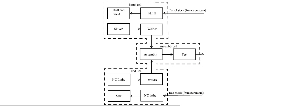
shows the three new JIT cells.

LESSON 2: CHANGING OVERHEAD TO DIRECT CELL ACTIVITIES COSTS.

While redesigning the machine operations, the cell workers wanted to know the costs of each machine task. This information could be used to measure the costs of scrap and rework, as well as providing bench­marks for productivity improvement over time (i.e., these are nonvalue-added activities). By summing the costs of each machine operation, the cost of making a cylinder barrel could be developed.

Since a kanban system controlled cylinder production, each cylinder kanban could be treated as a job. Thus, the team believed that a JOCAS would best provide the actual costs of making a cylinder. They dis­covered, however, that many production problems (causing cost variances) were cell related. Such prob­lems, and their cost variances, should not be treated as a cost of a particular cylinder (job) in the accounting system. Since 35,000 of the anticipated 40,000 cylinders to be produced in a year were identi­cal, the planners concluded that a standard PCAS should be used. Only part of the barrel cell's standard cost card is illustrated in Exhibit 8-20.   

   

Any of the overhead costs that were directly related to labor time were included within the worker's stan­dard price. For example, in the operating, inspecting, and move time allowed for “Machine Operation 1” of the standard cost card, the $10.65 per hour standard labor rate included a gross wage rate of $8.00 plus fringe benefits and payroll taxes of $2.65 per hour

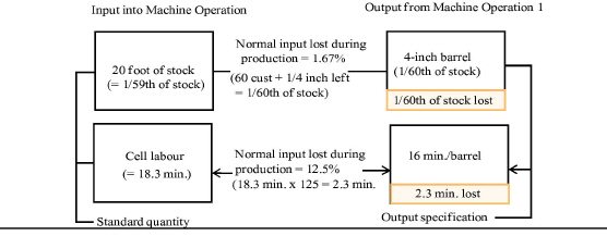
 The labor standard quantity included an allowance for miscellaneous time (e.g., breaks, setup, cleanup) of one hour per day. The scrap that could not be avoided was included in the barrel's direct material standard quantity. The following illustrates the standard quan­tity calculations:

One important aspect was separately including the cost of inspection time after each machine operation within the barrel's standard cost. World-class manufacturing and AT philosophies recognize the need for quality control when tasks are performed. The costs of “direct technology” (the costs of operating the machines) were also treated as direct costs within the cell. For example, machinery depreciation was based on operating time (depreciation was changed from a straight-line method to a rate per minute), as was machinery power cost.

LESSON 3: USE STANDARD ACTIVITY-BASED COSTS TO CALCULATE COST VARIANCES. Within the barrel cell (Exhibit 8-19), there are 4 machine operations. Each machine operation is considered as an activity. The activity-based standard costs now become the basis for computing cost variances and reconciling the actual costs incurred within the barrel cell each week. As a problem occurred, the cell worker coded it by activity for input into the cost management system. Having workers code the sources and causes and whether the problem has been corrected for input into the SCAS is not a new idea.²³ For example, one completed barrel had to be scrapped during the week. From the standard cost card, its incre­mental standard cost was $21.00. Also, one partially completed barrel had to be scrapped alter it was cut in Machine Operation 1. From the standard cost card, the cost of processing the barrel to this stage should be $5.25 (this production activity's standard cost). These are the third and fourth cost variances shown on the weekly report in Exhibit 8-21 

  

The control team at Newmount Engine Manufacturing believed it was important to understand the costs of production problems. Thus, when calculating and reporting cost variances, each variance was identified in terms of the activity that caused it. At the same time, cost variances could still be summarized in terms of materials, labor, and overhead, as in a traditional SCAS. To trace cost variances to their underlying prob­lems, however, the cell workers needed to identify those problems and code the input information by activ­ity for the cost management system. Because cost variances were coded and reported in terms of production activities, the Newmount cell workers called this an “activity-based cost variance reporting sys­tem.”

Attributes Needed For A Standard Cost Report

Assuming you are in a company with a relational database driven accounting system, what attributes do you need to add to the basic database tables in order to produce the Standard Cost reports? Using the generic REA template in Exhibit 5-22 to work on your answer. Include both the attribute and the table it would be from.

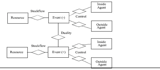
Summary Of Learning Objectives

The major goals of this chapter were to enable you to achieve six learning objec­tives:

Learning objective 1. Discuss the role of a standard cost accounting system (SCAS) in responsibility accounting.

Three responsibility accounting concepts are critical in designing an SCAS. First, standards must be designed jointly by management and operational personnel. Management involvement is needed to assure that the enterprise's goals are incorporated into the standards. Operational personnel must be involved so that they clearly understand what is expected. When employees participate in setting the standards used to evaluate their performance, they are more likely to accept the standards as legitimate and internalize the expected performance.

Standards and cost variances should not be the only basis for performance evaluation, though. In world-class enterprises, employees are rewarded for additional skills learned, preventive maintenance, sugges­tions for improvements, and the like. Primarily, an SCAS should provide the information needed to help people identify problems and correct them as soon as possible. The learning that results from control activities can prevent problems from happening in the future.

The second concept concerns the tightness of the standards. If ideal standards are set, unfavorable vari­ances will be common. Small unfavorable variances can signal excellent performance. With practical stan­dards, both favorable and unfavorable variances may suggest abnormal operating conditions. The SCAS should also report trend analysis over time for continuous improvement evaluation.

The third concept involves implementing the management-by-exception philosophy. Two issues are involved. First, when should variances be reported? To support quality control throughout the production process, variance information needs to be available on the shop floor in real time. An ICBIS and visual factory control system, with terminals at workstations, can provide immediate feedback and feedforward information to the workers. The input coding activities to identify the sources and causes of cost variances when they happen is the key idea for SCAS design in promoting effective and efficient operational con­trol.

The second issue involves which variances should be investigated. Some variances are investigated only if they fall outside preset control limits. Random fluctuations in labor time are often expected causing minor favorable and unfavorable variances that can be ignored. Other variances, such as problems with materials quality or machine breakdowns, are investigated whenever they occur and regardless of their significance. Exhibit 8-1 highlights the operational control loop and the steps involved in designing an SCAS for responsibility accounting.

Learning objective 2. Explain the meaning of a cost variance, and calculate and interpret the variable costs' spending variances.

The two basic types of cost variances are spending and usage. Cost variances compare standard prices and quantities against actual prices and quantities. Favorable variances result from actual costs being less than standard costs. When actual costs exceed standard costs, unfavorable variances result. The terms favorable and unfavorable refer to the effect on planned profits due to the cost variance. Favorable variances mean actual profits are greater than planned profits for the actual production volume. Unfavorable variances mean that actual profits are less than planned profits. In this way, variances measure the difference between planned and actual profits because of the activities that created those variances. Exhibit 8-5 summarizes the cost variance formulas and Demonstration Problem 1 presents the calculations and journal entries.

Spending variances for variable cost elements arc calculated with the following formula:

Variable cost spending variance

= Actual quantity purchased x (Standard price - Actual price)

A favorable direct materials spending (price) variance means the actual purchase price of direct materials is less than the standard price. Similarly, a favorable direct labor rate variance means the actual labor rate is less than the standard rate. The analysis of overhead variances can be performed by calculating one total overhead variance, or by calculating two, three, or four variances. Four-way overhead variance analysis provides better information than the other methods. Using the four-way method, separate spending and usage variances are calculated for VOH and FOH. The VOH spending variance has a limited interpretation in that it includes both price and usage problems.

Learning objective 3. Calculate and interpret the variable costs' usage variances.

The variable costs' usage variances can be calculated with the following formula:

Variable cost usage variance:

= Standard price x (Standard quantity allowed - Actual quantity used)

An unfavorable direct materials usage variance results from the actual quantity of materials used being greater than the standard quantity allowed (SQA). SQA is the total quantity of a manufacturing input that should have been used for the actual output. If the actual labor hours worked exceed the standard labor hours allowed, an unfavorable labor efficiency variance results. The VOH efficiency variance measures the difference between the SQA of the overhead application basis and the actual quantity used. To clarify this, let the POR's basis be machine usage. If more machine hours were used than should have been for the actual production volume (the standard machine hours allowed), an unfavorable VOH efficiency variance results. The assumption is that if more machine hours are worked, more variable overhead items are used. This may, or may not, be true.

Learning objective 4. Calculate and interpret the fixed overhead variances.

The four-way method of analyzing overhead cost variances provides separate FOH spending and usage variances. The FOH spending variance is called the budget variance. It measures the difference between the total budgeted FOH and the total actual FOH costs. in budgeting, control, and evaluation, fixed costs need to be considered as total costs, not as per unit costs. The per unit fixed cost is not stable over the rele­vant range. As production volume increases, the FOH per unit decreases. Fixed costs are stable (i.e., they have predictive usefulness) when measured as total costs. The formula for the FOR budget variance is:

FOR budget variance = Budgeted FOR cost - Actual FOH cost

The FOH usage variance (the volume variance) is a gauge of how well the factory is used. In interpreting this variance, FOR represents the costs of having the factory (the productive capacity) available for use. If the production quota is met, the factory is used as efficiently as planned. If the production quota is not obtained, the factory is not used as efficiently as planned when the FOR standard cost and the product's sales price were determined.

The interpretation of the FOR volume variance depends on the production volume used in the FOR stan­dard cost. The explanation above is valid when the production quota (the expected capacity) is used in pre­paring the standard cost card. The FOR volume variance formula is:

FOR volume variance = FOR standard cost x (Actual output - Budgeted output)

Exhibit 8-5 provides a variation of this formula, using the FOH POR basis (i.e., using units of input such as direct labor hours, instead of the above formula which uses units of output).

Learning objective 5. Prepare the journal entries for an SCAS, and the cost vari­ance report.

The cost variance calculations can be prepared and reported separately from the journal entries in an SCAS or both can be done together, as illustrated in Demonstration Problem 1. Cost elements are journal­ized into inventories using their standard costs. For example, direct materials are debited to RMI at their standard prices. When used, direct materials, direct labor, VOH and FOR are journalized into WIP at their standard

costs allowed (standard price x SQA, or standard cost x actual output). Actual costs are credited to accounts payable (for direct materials purchased), gross wages (for direct labor), and the VOA and FOE control accounts. The differences between the standard costs (debited) acid the actual costs (credited) arc recorded in separate subsidiary ledger accounts for the cost variances.

SCAS reports present cost variances in three ways. Cost variances per unit facilitate use by operations per­sonnel who often think about prices per pound, wage rates per hour, and pounds or hours per unit of prod­uct. Cost variance amounts reported in total dollars measure the difference between planned and actual profits, useful in profitability evaluations by upper management. Finally, cost variances as a percentage of standard help upper management and operations personnel judge their significance.

Learning objective 6. Design a high-quality SCAS with management reports useful for operational control and performance evaluation.

The modern management accountant has two roles in operational control and performance evaluation. First, an SCAS should provide the information wanted by different people in the firm. Second, if this is not perceived by the management accountant as the best (optimal) information, he or she must educate and demonstrate how different information can lead to better decisions. This second role is critical to the long-run success of the firm and its quest toward continuous improvement. Many traditional SCASs were designed primarily from a financial accounting perspective. Consequently, the historical usefulness of SCASs in operational control and performance evaluation has been quite limited.

Even in world-class enterprises, an SCAS may operate independently of the control system, or as an inte­gral component of it. For example, a simple backflush accounting system does not report information about cost variance problems for shop floor control or performance evaluation. Consequently, it cannot provide information useful in future planning activities. A separate information system is needed if control information is desired. On the other end of the SCAS design continuum is a production activity-based cost variance reporting system. This SCAS, using cause-effect coding of cost variances, provides online, real-time information for operational control, as well as for performance evaluation and future budgeting.

For effective and efficient operational control, the SCAS should report the sources and causes of cost vari­ances. Capturing information on the underlying activities that cause cost variances can provide valuable information both for short-run corrective actions as well as for long-run continuous improvement pro­grams. For example, favorable variances are not necessarily “good news.” A favorable direct materials spending variance may occur because substandard materials are purchased. When laborers use substan­dard materials, other variances result, such as unfavorable direct materials, direct labor, and VOH usage variances. Thus, one underlying cause of a particular variance also may be the cause of a number of other variances. In understanding production problems, these cause-effect chains must be identified. Develop­ing a database of historical cause-effect chains and the costs of corrective actions can aid in future opera­tional control decisions.

Learning objective 7. Prepare a list of attributes needed in a relational database to prepare Standard Cost reports in an REA environment.

Developing a Standard Cost Accounting System in a relational database involves adding a number of attri­butes to the basic tables and writing the reports. These should be seen as extensions of the basic model.

Important Terms

Backflush cost accounting system (BCAS) An SCAS that records input acquisitions at actual cost and output at standard cost. RMI is replaced with RIP, WIP is not used, and direct labor and overhead costs are debited to a Conversion Costs account. Input usage is recorded through the COGM or COGS journal entry, resulting in input costs being flushed backward out of the general ledger.

Direct labor efficiency variance This cost variance is the difference between the standard direct labor hours allowed and direct labor hours used, multiplied by the standard rate per direct labor hour. It measures the difference between planned and actual production labor costs due to labor efficiency being more or less than what it should have been for the actual output.

Direct Labor mix variance This variance measures the difference in the average standard price of labor from assigning workers to activities in a manner different from planned. Thus, it is a spending variance.

Direct labor rate variance This variance reports the difference between the standard direct labor rate and the actual direct labor rate per hour, multiplied by the actual direct labor hours worked. It mea­sures the difference in labor costs from budget due to changes in wage rates and/or payroll taxes and fringe benefits.

Direct labor yield variance This variance presents the difference between planned and actual profits from the use of a different mix of labor than originally planned. Thus, it is a usage variance.

Direct materials mix variance This variance measures the change in the average standard price from mixing direct materials in a ratio different from the standard direct materials formula. Thus, it is a price variance.

Direct materials price variance This variance reports the difference between the standard price and the actual price, multiplied by the actual quantity of direct materials purchased. It measures the differ­ence in direct materials costs from budget due to price differences from standard.

Direct materials usage variance This variance is the difference between the standard quantity allowed and the actual quantity of direct materials used, multiplied by the standard price. It measures the difference in direct materials cost from the standard cost allowed due to usage of direct materials.

Direct materials yield variance This variance is the result of obtaining an output different from the one expected based on the total quantities of direct materials used. It measures the impact on planned profits from the difference between the total quantity of materials that should have been used with the standard mix and the actual total quantity of direct materials used. Thus, it is a usage variance.

Favorable cost variance A favorable variance results when actual costs are less than standard costs allowed. A spending variance is favorable when the actual price of an input item is less than its standard price. A favorable usage variance results when the actual quantity used is less than that input's standard quantity allowed.

Fixed overhead budget variance This variance is the difference between the budgeted fixed overhead costs and the actual fixed overhead costs.

Fixed overhead volume variance This variance measures the difference between budgeted profits and actual profits created by producing a different volume than planned.

Flexible budget A budget that is prepared using the actual production volume rather than the production quota. It can be used to compare actual and “should be” variable costs for the same level of pro­duction.

Raw-in-process (RIP) The general ledger account for raw materials purchased in a BCAS. Raw materials costs are removed from this account at the completion or sale of the products.

Standard cost allowed (SCA) The total cost of an input that should have been incurred for the actual out­put. It is calculated by multiplying an input's standard cost and actual production volume, or by multiplying standard price and standard quantity allowed for that input.

Standard quantity allowed (SQA) The total amount of an input item that should have been used given the actual output produced. it is the result of multiplying an input's standard quantity by the actual production volume.

Total overhead variance This is simply the sum of the four overhead cost variances. It is also the differ­ence between the total overhead costs applied and the total overhead costs actually incurred.

Unfavorable cost variance An unfavorable variance results when actual costs are greater than standard costs. An unfavorable spending variance occurs when the actual price of a cost element is greater than its standard price. When the actual input quantity is greater than its standard quantity allowed, an unfavorable usage variance results.

Variable overhead efficiency variance This variance measures the difference between the standard quan­tity allowed of the basis used to apply VOH costs and the actual quantity used. When direct labor hours are used to apply VOH, then an unfavorable labor usage variance causes an unfavorable VOH usage variance.

Variable overhead spending variance This variance is the difference between the VOH standard price multiplied by the actual quantity of the overhead application basis used and the actual total VOH costs. It measures the difference between total actual VOH cost and the VOH cost that should have been incurred given the number of direct labor hours worked (or the actual quantity of the basis used to apply overhead if it is something other than direct labor hours).

Demonstration Problems

DEMONSTRATION PROBLEM 1 Calculating cost variances and preparing SCAS journal entries.

Armando Corporation manufactures electronic video and audio equipment. Each of its products is made in a separate department. One of its newer products, CD Players, is built in the CD Player Department. CD Players are made one-at-a-time in quality circles. To further control quality and reduce inventory costs, the department operates on a AT basis. Thus, there are no beginning or ending WIP inventories. Armando has two overhead accounts (variable and fixed), and direct labor hours is the cost driver for both. Armando uses an SCAS with monthly cost variance reports issued for each department.

Two data sections follow. The CD Player standard absorptive manufacturing cost is $93. Normal produc­tion volume requires 2,400 direct labor hours per month.

 

Required:

Prepare the journal entries to record direct materials purchases, usage of direct materials and labor, and applied VOH and FOH. Also record the cost of CD Players completed.

SOLUTION TO DEMONSTRATION PROBLEM 1 

 

Before preparing the input usage journal entries, the following calculations are needed:

SQ_{Direct materials}: 19 lb. / (1.00 - .05)    = 20 lb. per unit

SQ_{Direct labour}: 3.60 DLhr / (1.00 - .10)    = 4 DLhr per unit 

SQA_{Direct materials}: 20 lb. per unit x 500 units    = 10,000 lb.

SQA_{Direct materials}: 4 DLhr per unit x 500 units    = 2,000 DLhr

    

    

   

  

DEMONSTRATION PROBLEM 2 - Preparing the standard cost card, manufacturing cost equation, and cost variance report.

Using the two data sections from Demonstration Problem 1:

(a) prepare the standard cost card and manufacturing cost equation using the format from Exhibit 8-11, and

(b) prepare a cost variance report using the format from Exhibit 8-12

SOLUTION TO DEMONSTRATION PROBLEM 2

  

 

Review Questions

8.1    Explain how an SCAS is applicable in an enterprise that routinely manufactures the same products or performs the same services. Are standard costs and cost variances applicable to companies that make an array of unique products or perform one-of-a-kind services? Are standard costs and cost variances useful for construction companies, consultants, repair shops, and hospitals?

8.2    What is the difference between an SCAS and a normal or actual CAS?

8.3    How does a favorable variance differ from an unfavorable variance?

8.4    What is meant by the term “management-by-exception”? Explain how it is used in an SCAS. Dis­cuss how it may be misused.

8.5    Why is it important to consider how standards are set? Which type of standards do you believe will better motivate employees, ideal or practical? Why?

8.6    Is it important to present trend analyses of standards and/or variances over time? Why isn't it suffi­cient to just report cost variances each period?

8.7    Do favorable variances always represent “good” performance? Do unfavorable variances always represent “bad” performance?

8.8    List and very briefly describe the steps in variance analysis and operational control.

8.9    What is the “key” factor for operational control?

8.10    In world-class enterprises, when are operational control actions taken?

8.11    Should the SCAS provide feedforward information in support of operational control? Explain your answer.

8.12    How can an SCAS reduce record-keeping costs?

8.13    Distinguish between the two basic types of cost variances.

8.14    List the four formulas for the eight cost variances.

8.15    What are three possible underlying causes of direct materials price variances?

8.16    What are three possible underlying causes of direct labor rate variances?

8.17    Explain a VOH spending variance. Why is it important to break down this variance into its individ­ual items?

8.18    Define and give an example of a flexible budget.

8.19    What is meant by the term “standard quantity allowed”?

8.20 Which responsibility center is customarily held responsible for an unfavorable direct materials usage variance? What are three possible underlying causes of direct materials usage variances?

8.21    What are three possible underlying causes of direct labor efficiency variance? Why is it important to investigate this variance?

8.22    Explain three characteristics that a high-quality SCAS should possess.

8.23    Explain the VOH efficiency variance.

8.24    What is the difference between the FOH budget and volume variances? Are these really spending and usage variances?

8.25    How does the production volume used in determining the FOH standard cost affect the interpreta­tion of the FOH volume variance?

8.26    What are the differences between the two-way variance analysis method and the three-way variance analysis method?

8.27    The total production overhead variance can be divided into two, three, or four variances. No matter how many variances are isolated, one is always the:

   a. Flexible budget variance,

   b. Fixed overhead volume variance.

   c. Variable overhead efficiency variance.

   d. Variable overhead spending variance.

8.28    Explain the two basic differences between SCAS journal entries and PCAS or JOCAS journal entries.

8.29    In designing the SCAS general ledger system for WIP, what type of accounts are cost variances? Why are cost variance accounts organized by responsibility center?

8.30    Identify two differences between the journal entries in a standard PCAS and in a standard JOCAS.

8.31    How should variances of significant amounts be treated at the end of the accounting period?

   a. Reported as a different charge or credit.

   b. Allocated among work-in-process inventory, finished goods inventory, and cost of goods sold.

   c. Charged or credited to cost of goods manufactured.

   d. Allocated among cost of goods manufactured, finished goods inventory, and cost of goods sold.

8.32    Why do cost variances need to be reported in total, per unit, and as a percentage of standard? How are these different calculations useful to different people within the enterprise?

8.33    Distinguish between:

   Direct materials mix variance

   Direct materials yield variance

   Explain the purpose of each. Together, what variance do they comprise?

8.34    Distinguish between:

   Direct labor mix variance

   Direct labor yield variance

   Explain the purpose of each. Together, what variance do they comprise?

8.35    How does a BCAS differ from a traditional SCAS?

8.36    How does a production activity-based SCAS differ from a traditional SCAS?

8.37    Why is it important to identify cost variances in terms of the underlying activities that create them?

Chapter-specific Problems

These problems require responses based directly on concepts and techniques presented in the text.

8.38 Entry in the accounts for direct materials variances. At Timken Company during August direct materials were purchased for $650 (at $5 per square foot). Their standard price is $4. In project 738A, 1,000 square feet of materials were used. According to standards, 900 square feet should have been used.

Calculate the direct materials cost variances and make the journal entries.

8.39 Entry in the accounts for direct labor variances. Project 738A at Timken Company (see the previ­ous problem) also required 50 direct labor hours to complete at a rate of $10 per hour, when it should have taken only 45 hours at a rate of $12 per hour.

Required: Make the journal entries for the direct labor usage on project 738A.

8.40 Solving for the actual direct materials purchase price. [AICPA adapted] Information Oil Kennedy Company's direct materials costs includes:

Required: Calculate the actual purchase price rounded to the nearest penny.

8.41 Solving for the standard and actual direct labor rates. [AICPA adapted] Goodman Company's direct labor costs are as follows:

   Standard direct labor hours 30,000

   Actual direct labor hours 29,000

   Direct labor efficiency variance, favorable $4,000

   Direct labor rate variance, favorable $5,800

   Total gross wages $110,200

Required: 

a. What was Goodman's standard direct labor rate?

b. What was Goodman's actual direct labor rate?

8.42 Direct materials and labor variances. [CMA adapted] Arrow Industries employs a standard cost system. Arrow has established the following standards for the prime costs of its Hunters’ Bow product line:

 

During November, Arrow purchased 160,000 pounds of direct materials at a total cost of $304,000. The total factory wages for November were $42,000, 90% of which were for direct labor. Arrow manufactured 19,000 Hunters' Bows during November using 142,500 pounds of direct materials and 5,000 direct labor hours.

Required:

a. What was the direct materials purchase price variance for November?

b. What was the direct materials usage variance for November?

c. What was the direct labor rate variance for November?

d. What was the direct labor efficiency variance for November?

8.43 Direct labor variances (including mix and yield). [CMA adapted] Landeau Manufacturing Com­pany has a process cost accounting system. A monthly analysis compares actual results with both a monthly plan and a flexible budget. Standard direct labor rates used in the flexible budget are established at the time the annual plan is formulated and held constant for the entire year. Standard direct labor rates in effect for the fiscal year ending June 30 and standard hours allowed for the output in April are:

 

The wage rates for each labor class increased on January 1 under the terms of a new union contract negoti­ated in December of the previous fiscal year. The standard wage rates were not revised to reflect the new contract. The actual direct labor hours worked and the actual direct labor rates per hour experienced for the month of April were:

Required:

a. What is the total direct labor variance?

b. What is the direct labor rate variance?

c. What is the direct labor efficiency variance?

d. What is the direct labor yield variance? (Round all standard prices to four decimal places.)

e. What is the direct labor mix variance for April?

8.44 Applied overhead and overhead usage variances. [AICPA adapted] Union Company uses a standard cost accounting system. The following overhead costs and production data are available for August:

 

Required:

a. What should be the amount of applied overhead for August?

b. Calculate the VOH efficiency variance.

c. Calculate the FOH volume variance.

8.45 Spending variance using the three-way variance analysis method. [AICPA adapted] The following information is available from the Tyro Company:

 

Required:

Assuming that Tyro uses a three-way variance analysis method, what is the spending variance?

8.46 Fixed overhead production volume variance using the two-way variance analysis method. [AICPA adapted] Information on Ripley Company's overhead costs for the January production activity is as fol­lows:

 

Required:

Using the two-way variance analysis method, calculate the FOB production volume variance for January. Will the three-way variance analysis method produce the same FOH production volume variance? Explain.

8.47 Flexible budget controllable variance. [CMA adapted] Universal Company uses a standard cost sys­tem and has prepared the following budget at normal capacity for the month of January:

 

Actual data for January were as follows:

 

Required: Using the two-way variance analysis method, calculate the flexible budget controllable variance for January.

8.48 VOH and FOH variances and journal entries. [AICPA adapted] Based on a monthly normal volume of 50,000 units (100,000 direct labor hours), Raff Company's standard cost system contains the following overhead costs for department A:

• Variable   $6 per unit

• Fixed   $8 per unit

The following information pertains to the month of March:

• Units actually produced   38,000

• Actual DLhr worked   80,000

Actual overhead incurred:

• Variable   $250,000

• Fixed   384,000

Required:

a. Calculate the VOH spending variance for March.

b. What is the VOH efficiency variance?

c. Determine the FOH budget variance.

d. Calculate the FOH volume variance for March.

e. Prepare the journal entries to record VOH and FOH.

8.49 Four production overhead variances and journal entries. [CMA adapted] Derf Company applies overhead on the basis of direct labor hours in department B. Two direct labor hours are required for each product unit. Planned production for the period was set at 9,000 units. Manufacturing overhead was bud­geted at $135,000 for the period; 20% of this cost is fixed. The 17,200 hours worked during the period resulted in production of 8,500 units. Variable manufacturing overhead costs incurred were $108,500, and fixed manufacturing overhead costs were $28,000. Derf Company uses a four-variance method for analyz­ing manufacturing overhead.

Required:

a. Calculate the VOH spending variance for the period.

b. Calculate the VOH efficiency variance for the period.

c Calculate the FOH spending (budget) variance for the period.

d. Calculate the FOH production volume variance for the period.

e. Prepare the journal entries to record VOH and FOH.

8.50 Four production overhead variances and journal entries. [CMA adapted] Franklin Glass Works' production budget for the year ended November 30, 20x4, in department C was based on 200,000 units. Each unit requires two standard hours of labor for completion. Total overhead was budgeted at $900,000 for the year, and the fixed overhead rate was estimated to be $3 per unit. Both fixed and variable overhead are applied to the product on the basis of direct labor hours. The actual data for the year ended November 30, 20x4, are as follows:

 

Required:

a. What were the standard hours allowed for actual production for the year ended November 30, 20x4?

b. What was the VOH efficiency variance for the year?

c. What was the VOH spending variance for the year?

d. What was the FOH spending variance for the year?

e. What was the FOH applied to Franklin's production for the year?

f. What was the FOH production volume variance for the year?

g. Prepare the VOH and FOB journal entries.

8.51 Multiple direct materials, mix and yield variances. [CMA adapted] Energy Modification Company produces a gasoline additive, Gas Gain. This product increases engine efficiency and improves gasoline mileage by creating a more complete burn in the combustion process. Careful controls are required during the production process to ensure that the proper mix of input chemicals is achieved and that evaporation is controlled. Loss of output and efficiency may result if the controls are not effective. The standard cost of producing a 500-litre batch of Gas Gain is $135. The standard materials mix and related standard cost of each chemical used in a 500-litre batch are as follows:

 

The quantities of chemicals purchased and used during the current production period are shown in the schedule below. A total of 140 batches of Gas Gain were manufactured during the current production period. Silly Willy, the controller of Energy Modification Company, determines its costs and chemical usage variations at the end of each production period.

  

Required:

a. What is the direct materials purchase price variance for Echol?

b. What is the direct materials purchase price variance for Protex?

c. What is the direct materials purchase price variance for Benz?

d. What is the direct materials purchase price variance for CT-40?

e. What is the direct materials usage variance for Echol?

f. What is the direct materials usage variance for Protex?

g. What is the direct materials usage variance for Benz?

h. What is the direct materials usage variance for CT-40?

i. What is the direct materials mix variance?

j. What is the direct materials yield variance?

8.52 Comprehensive direct labor variance analysis. [CMA adapted] Mountain View Hospital has adopted a standard cost accounting system for evaluation and control of nursing labor. Diagnosis Related Groups (DRGs), instituted by the U.S. government for health insurance reimbursement, are used as the output measure in the standard cost system. A DRG is a patient classification scheme that treats hospitals as multipartite firms; in-patient treatment procedures are related to the numbers and types of patient ail­ments treated. Mountain View Hospital has developed standard nursing times for the treatment of each DRG classification, and nursing labor hours are assumed to vary with the number of DRGs treated within a time period.

The nursing unit on the fourth floor treats patients with four DRG classifications. The unit is staffed with registered nurses (RNs), licensed practical nurses (LPNs), and aides. The standard nursing hours and sal­ary rates for the nursing unit are as follows:

The results of operations for the fourth-floor nursing unit for the month of May 20x4, arc presented below:

 

 

The time accountant for Mountain View Hospital calculated the following standard times for the fourth-floor nursing unit for May 20x4:

 

Since the hospital does not have data to calculate variances by DRG, it calculates labor variances, using a flexible budgeting approach, for each reporting period by labor classification (RN, LPN, Aide). Labor mix and labor yield variances are also calculated since one labor input can be substituted for another labor input. The variances are used by nursing supervisors and hospital administration to evaluate the perfor­mance of nursing labor.

Required:

a. Calculate the total flexible budget variance for the fourth-floor nursing unit of Mountain View Hospital for May 20x4, indicating how much of this variance is attributed to:

1. Labor efficiency.

2. Rate differences:

b.

1. Calculate the labor mix variance for the fourth-floor nursing unit of Mountain View Hospital (Use whole hours and whole cents in all calculations.)

               2. Explain the significance of the labor mix variance calculated in Requirement 2.(b)1.

c.

1. Calculate the labor yield variance for the fourth-floor nursing unit of Mountain View Hospital. (Use whole hours and whole cents in all calculations.)

2. Interpret the meaning of the labor yield variance calculated in Requirement (c)1.

8.53 Comprehensive direct materials and labor variances analysis. Dash Company adopted a standard cost system several years ago. The standard costs for the prime costs of its single product are as follows:

Direct materials (8 kilograms x $5.00/kg)   $40.00

Direct labor (6 hours x $8.201hr)   $49.20

The operating data for November are:

• In-process beginning inventory: None.

• In-process ending inventory: 800 units, 75% complete as to labor; material is issued at the beginning of processing.

• Units completed: 5,600 units.

• Budgeted output: 6,000 units.

• Purchases of materials: 50,000 kilograms.

• Total actual direct labor costs: $300,760.

• Actual hours of labor: 36,500 hours

• Direct materials usage variance: $1,500 unfavorable.

• Total direct materials variance: $750 unfavorable.

Required: Calculate the..

a. direct labor efficiency variance for November.

b. direct labor rate variance for November.

c. actual kilograms of direct materials used in production during November.

d. actual price paid per kilogram of direct materials during November.

e. total amounts of direct materials and labor costs transferred to the finished goods account for November.

f. total amount of direct materials and labor costs in the ending balance of WIP inventory at the end of November. [CMA adapted]

8.54 Direct materials, labor, and overhead variances. [CMA adapted] Eastern Company manufactures special electrical equipment and parts. Eastern employs a standard cost accounting system with separate standards established for each product.

A special transformer is manufactured in the Transformer Department. Production volume is measured by direct labor hours in this department, and a flexible budget system is used to plan and control department overhead.

Standard costs for the special transformer are determined annually in September for the coming year_ The standard cost of a transformer for the year was computed at $67 as follows:

 

Overhead rates were based upon normal and expected monthly capacity for the year, both of which were 4,000 direct labor hours. Practical capacity for this department is 5,000 direct labor hours per month. Vari­able overhead costs are expected to vary with the number of direct labor hours actually used.

During October, 800 transformers were produced. This was below expectations because a work stoppage occurred during contract negotiations with the labor force. Once the contract was settled, the department scheduled overtime in an attempt to catch up to expected production levels.

The following costs were incurred in October:

Overtime: 600 of the 1,400 hours were subject to overtime premium. The total overtime premium of $2,160 is included in variable overhead in accordance with company accounting practices.

Variable overhead:   $10,000

Fixed overhead:   $ 8,800

Required:

a. When is the most appropriate time to record any variance of actual direct materials price from standard? Explain your answer.

b. Calculate the direct labor rate variance.

c. Calculate the total direct materials usage variance.

d. Calculate the VOH spending variance.

e. What are the number of hours used to calculate the VOH efficiency variance?

f. Calculate the FOH spending variance.

g. Calculate the FOH production volume variance.

8.55 Comprehensive problem for direct materials, labor, and overhead variances. [AICPA adapted] Gelltite Corporation manufactures a basic line of draperies with the following standard costs:

Standards are based on normal monthly production involving 2,400 direct labor hours (600 units of out­put).

The following information pertains to the month of July:

Direct materials purchased (18,000 yards x $1.38 per yard)    $24,840

Direct materials used    9,500 yards

Direct labor (2,100 hours x $9.15 per hour)    $19,215

Actual factory overhead    $16,650

500 units of the product were actually produced in July.

Required:

a. Calculate the predetermined VOH rate per direct labor hour.

b. Calculate the budgeted FOH costs based on normal activity.

c. Calculate the direct materials price variance (isolated at time of purchase).

d. Calculate the direct materials usage variance for July.

e. Calculate the direct labor rate variance for July.

f. Calculate the direct labor efficiency variance for July.

g. Calculate the total budgeted overhead costs.

h. Calculate the total applied factory overhead costs.

i. Calculate the FOH production volume variance.

8.56 Comprehensive flexible budgeting and variance analysis. Cain Company has an automated pro­duction process, and consequently, machine hours are used to describe production activity. A full absorp­tion costing system is employed by the company. The annual profit plan for the coming fiscal year is finalized in April of each year. The profit plan for the fiscal year ending May 31 called for 6,000 units to be produced, requiring 30,000 machine hours. The full absorption costing rate for the fiscal year was deter­mined using 6,000 units of planned production.

Cain develops flexible budgets for different levels of activity for use in evaluating performance. A total of 6,200 units was actually produced during the fiscal year requiring 32,000 machine hours. The schedule presented below (in both columns) compares Cain Company's actual costs for the fiscal year with the profit plan and the budgeted costs for two different activity levels. Cain uses the three-way variance analysis method. The report below is in thousands of dollars.

 

Required:

a. Calculate the actual cost of direct materials used in one unit of product.

b. Calculate the cost of direct materials that should be processed per machine hour.

c. Calculate the budgeted direct labor cost for each unit produced.

d. Calculate the variable manufacturing overhead rate per machine hour in a flexible budget formula

e. Calculate the FOH production volume variance for the year.

f. Calculate the overhead spending variance for the year.

g. Calculate the VOH efficiency variance for the year.

h. How much overhead was applied to finished goods?

i. What is the total overhead variance?

j. Using the flexible budget formula, calculate the total budgeted manufacturing costs (in thousands of dol­lars) for an output of 6,050 units. [CMA adapted]

Think-tank Problems

Although these problems are based on chapter material, reading extra material, reviewing previous chap­ters, and using creativity may be required to develop workable solutions.

8.57 Allocation of variances. [AICPA adapted] Tolbert Manufacturing Company uses a standard cost sys­tem in accounting for the cost of production of its only product, product A. The standards for the produc­tion of one unit of product A are as follows:

• Direct materials: 10 feet of item 1 at $0.75 per foot and 3 feet of item 2 at $1 per foot.

• Direct labor: 4 hours at $3.50 per hour.

• Manufacturing overhead: Applied at 150% of standard direct labor costs.

There was no inventory on hand at the beginning of the year. Material price variances are isolated at pur­chase. Following is a summary of costs and related data for the production of product A during the year:

• 100,000 feet of item 1 were purchased at $0.78 per foot.

• 30,000 feet of item 2 were purchased at $0.90 per foot.

• 8,000 units of product A were produced, which required 78,000 feet of item 1; 26,000 feet of item 2; and 31,000 hours of direct labor at $3.60 per hour.

• 6,000 units of product A were sold.

Required:

a. What should be the total debits to the materials inventory account for the purchase of item 1?

b. What should be the total debits to the WIP inventory account for direct labor?

c. What is the balance in the direct materials usage variance account for item 2?

d. If all standard variances are allocated to cost of goods sold and inventory accounts, what is the amount of direct materials usage variance for item 2 to be allocated to the materials inventory account?

e. If all standard variances are allocated to cost of goods sold and inventory accounts, what would be the amount of direct materials price variance of item l to be allocated to the materials inventory account?

8.58 Comprehensive analysis of variances. [CMA adapted] Allglow Company is a cosmetics manufac­turer specializing in stage makeup. The company's best-selling product is SkinKlear, a protective cream used under the stage makeup to protect the skin from frequent makeup use. SkinKlear is packaged in three sizes-8 ounces, one pound, and three pounds-and regularly sells for $21 per pound. The standard cost per pound of SkinKlear, based on Allglow's_.normal monthly production of 8,000, pounds, is as follows:

 

Based on these standard costs, Allglow prepares monthly budgets. Following are the budgeted perfor­mance and the actual performance for May 20x6, when the company produced and sold 9,000 pounds of SkinKlear:

 

Barbara Simmons, Allglow's president, was not pleased with these results; despite a sizable increase in the sales of SkinKlear, the product's contribution to the overall profitability of the firm decreased. Simmons has asked Allglow's cost accountant, Brian Jackson, to prepare a report that identifies the reasons why the contribution margin for SkinKlear has decreased. Jackson has gathered the following information to help in the preparation of the report:

 

While doing his research, Jackson discovered that the Manufacturing Department had mechanized one of the manual operations in the compounding process on an experimental basis. The mechanized operation replaced manual operations that represented 40% of the compounding process.

The workers' inexperience with the mechanized operation caused increased usage of both the cream base and the moisturizer; however, Jackson believed these inefficiencies would be negligible if mechanization became a permanent part of the process and the workers' skills were improved. The idle time in compound­ing was traceable to the fact that fewer workers were required for the mechanized process. During this experimental period, the idle time was charged to direct labor rather than overhead. The excess workers could either be reassigned or laid off in the future. Jackson also was able to determine that all of the vari­able manufacturing overhead costs over standard could be traced directly to the mechanization process.

Required:

a. Prepare an explanation of the cost variances included in the $3,600 unfavorable variance between the budgeted and actual contribution margin for SkinKlear during May 20x6 by calculating the following vari­ances:

1. Material price variance.

2. Material quantity variance.

3. Labor efficiency variance.

4. Variable overhead efficiency variance.

5. Variable overhead spending variance.

b. Allglow Company must decide whether to continue the mechanization of the compounding operation in the SkinKlear manufacturing process that was mechanized on an experimental basis. Calculate the variable cost savings that can be expected to arise in the future from the mechanization. Explain your answer.

8.59 Motivational aspects and benefits of a standard cost system. [CMA adapted] Terry Travers is the manufacturing supervisor of the Aurora Manufacturing Company, which produces a variety of plastic products. Some of these products are standard items that are listed in the company's catalogue, while others are made to customer specifications. Each month, Travers receives a performance report displaying the budget for the month, the actual activity for the period, and the variance between budget and actual. Part of Travers's annual performance evaluation is based on her department's performance against budget. Aurora's purchasing manager, Bob Christensen, also receives monthly performance reports and is evalu­ated in part on the basis of these reports.

Last month's reports have just been distributed on the 21st of this month, when Travers met Christensen in the hallway outside their offices. Scowling, Travers began the conversation, “I see we have another set of monthly performance reports hand-delivered by that not very nice junior employee in the budget office. He seemed pleased to tell me that I was in trouble with my performance again.”

Christensen: “I got the same treatment. All I ever hear about are the things I haven't done right. Now, I'll have to spend a lot of time reviewing the report and preparing explanations. The worst part is that the information is almost a month old, and we spend all this time on history.”

Travers: “My biggest gripe is that our production activity varies a lot from month to month, but we're given an annual budget that's written in stone. Last month, we were shut down for three days when a strike delayed delivery of the basic ingredient used in our plastic formulation, and we had already exhausted our inventory. You know about that, of course, since we asked you to call all over the country to find an alter­nate source of supply. When we got what we needed on a rush basis, we had to pay more than we normally do.”

Christensen: “I expect problems like that to pop up from time to time-that's part of my job-but now we'll both have to take a careful look at the report to see where charges are reflected for that rush order. Every month, I spend more time making sure I should be charged for each item reported than I do making plans for my department's daily work. It's really frustrating to see charges for things I have no control over.”

Travers: “The way we get information doesn't help either. I don't get copies of the reports you get, yet a lot of what I do is affected by your department and by most of the other departments we have. Why do the budget and accounting people assume that I should only be told about my operations even though the pres­ident regularly gives us pep talks about how we all need to work together as a team?”

Christensen: “I seem to get more reports than I need, and I am never asked to comment until top manage­ment calls me on the carpet about my department's shortcomings. Do you ever hear comments when your department shines?”

Travers: “I guess they don't have time to review the good news. One of my problems is that all the reports are in dollars and cents. I work with people, machines and materials. I need information to help me this month solve this month's problems–not another report of the dollars expended last month or the month before.”

Required:

a. Based upon the conversation between Terry Travers and Bob Christensen, describe the likely motiva­tion and behavior of these two employees resulting from Aurora Manufacturing Company's variance reporting system.

b. Both employees and companies should benefit from properly implemented variance reporting systems.

1. Describe the benefits that can be realized from using a variance reporting system.

2. Based on the situation presented above, recommend ways for Aurora Manufacturing Company to improve its variance reporting system so as to increase employee motivation.

8.60 Developing standard costs and explaining the causes of variances. [CMA adapted] ColdKing Company is a small producer of fruit-flavored frozen desserts. For many years, ColdKing's products have had strong regional sales on the basis of brand recognition. However, other companies have begun market­ing similar products in the area, and price competition has become increasingly important. John Wake­field, the company's management accountant, is planning to implement a standard cost system for ColdKing and has gathered considerable information from his co-workers on production and material requirements for ColdKing's products. Wakefield believes that the use of standard costing will allow Cold­King to improve cost control and make better pricing decisions.

ColdKing's most popular product is raspberry sherbet. The sherbet is produced in ten-gallon batches, and each batch requires six quarts of good raspberries. The fresh raspberries are sorted by hand before entering the production process. Because of imperfections in the raspberries and normal spoilage, one quart of ber­ries is discarded for every four quarts of acceptable berries. Three minutes is the standard direct labor time for the sorting required to obtain one quart of acceptable raspberries. The acceptable raspberries are then blended with the other ingredients; blending requires 12 minutes of direct labor tune per batch. After blending, the sherbet is packaged in quart containers. Wakefield has gathered the following pricing infor­mation:

•  ColdKing purchases raspberries at a cost of $.80 per quart. All other ingredients cost a total of $.45 per gallon.

• Direct labor is paid at the rate of $9.00 per hour.

• The total cost of direct materials and direct labor required to package the sherbet is $38 per quart.

Required:

a. Develop the standard cost for the direct cost components of a ten-gallon batch of raspberry sherbet. The standard cost should identify the:

1. Standard quantity.

2. Standard rate.

3. Standard cost per batch for each direct cost component of a batch of raspberry sherbet.

b. As part of the implementation of a standard cost system at ColdKing, John Wakefield plans to train those responsible for maintaining the standards in the use of variance analysis. Wakefield is particularly concerned with the causes of unfavorable variances.

1. Discuss the possible causes of unfavorable direct materials price variances, and identify the individ­ual(s) who should be held responsible for these variances.

2. Discuss the possible causes of unfavorable direct labor efficiency variances, and identify the individ­ual(s) who should be held responsible for these variances.

8.61 Ethical considerations in SCAS design. Chapter 1 identified four ethical standards for management accountants. What are the implications of each standard in designing a high-quality SCAS?

8.62 Accounting for loss. Review the procedures involved in accounting for scrap, rework, and spoilage presented in Chapters 5, 6, and 7. Given the goal of designing a high-quality SCAS, create a policy to account for all three types of loss. Demonstrate how this policy works through an illustration of the journal entries in a ' PCAS and JOCAS.

8.63 High-quality information and SCAS design. Consider each characteristic of high-quality informa­tion presented in Chapter 1. What implications does each have in the design of a high-quality SCAS for use in either a process or job order situation?

8.64 SCAS for SIT. Design the WIP general ledger system for a JIT SCAS. The cost accounting system should be a high-quality system. Consider whether cost variance information is really needed. If so, how should the cost variances be calculated and reported? If you do not think cost variances information is needed, then what information should be provided by the SCAS, to whom, and how?

8.65 Backflush systems and production activity-based SCASs. In the chapter it was argued that these two types of SCASs represent opposite ends on a continuum of SCAS design sophistication. Do you agree? Why? Discuss the benefits and limitations of each type of SCAS.

8.66 Cost variances, journal entries, and reports. Another product Armando Corporation makes is a turntable (Armando Corporation was introduced in Demonstration Problems I and 2). The turntable also is made in its own department. As with CD Players, there are no beginning or ending WIP inventories. The department has two overhead accounts (variable and fixed) and direct labor hours is the cost driver for both. Armando uses a standard cost system with monthly cost variance reports issued for this department.

The turntable's standard absorptive manufacturing cost (SAMC) is $44. Fixed overhead in the department is budgeted at $120,000 per month. Following are the data for standard costs and actual activity during May:   

  

Required:

a. Calculate the cost variances for direct materials, direct labor, VOH and FOR and the total monthly cost variance for the department.

b. Journalize the cost variances and completed production transferred to FGI.

c. Prepare a report that presents the cost variances in total, per unit, and as a percentage of standard.

8.67 SCAS spreadsheet reports. Refer to the previous problem. Create a spreadsheet program that reports monthly cost variances. It should report each cost variance per unit, in total, and as a percentage. The report should also include both Data Sections and the Standard Cost Card. Use the format from Exhibits 8-11 and 8-12.

8.68 Cost variances, journal entries, and reports. Logan Boris Company is a subsidiary of Ben Logan Golf Club Corporation. Logan Boris makes metal woods and different types of irons, each in separate departments. The company maintains two over-head accounts (variable and fixed), and direct labor hours is the cost driver for both. All subsidiaries of Ben Logan use a standard cost system with annual cost vari­ance reports issued to corporate headquarters for each subsidiary company.

The standard absorptive manufacturing cost for a metal wood is $32 (the Data Section for the standard cost card is shown below). Last year, Logan Boris had a production quota of 10,000 metal woods, but pro­duced 11,000.

• The actual costs for last year were:

• Utilities: $500 for the sales office, $11,000 for the factory ($4,000 was considered a fixed cost).

• Insurance: $500 for the office, $2,000 for the factory.

• Depreciation: Factory = $10,000 (straight-line basis), office = $900.

• Salaries: Sales office = $50,000, factory supervision = $25,000.

• Advertising: $100,000.

• Finished clubs delivery expense: $10,000.

• Direct materials purchased: 50,000 pounds at $1.90/lb.

• Gross wages: Direct labor = $193,200 (23,000 DLhr worked), $35,000 indirect.

• Materials used: Direct materials = 35,000 lb., factory supplies = $20,000, office supplies = $1,000.

 

Required:

a. Calculate the cost variances for direct materials, direct labor, VOH and FOH, and the total annual cost variance for the department.

b. Journalize the cost variances and completed production transferred to FGI.

c. Prepare a report that presents the cost variances in total, per unit, and as a percentage of standard. To avoid rounding errors, input one-sixth as the normal input loss percentage (instead of 16.67%) shown in the Data Section.

8.69 SCAS spreadsheet reports. Refer to the previous problem. Create a spreadsheet program that reports annual cost variances. It should report each cost variance per unit, in total, and as a percentage. The report should also include both Data Sections and the Standard Cost Card. Use the format from Exhibits 8-11 and 8-12.