Chapter 18  :  Analyzing Cost-volume-profit Relationships

LEARNING OBJECTIVES

After studying this chapter, you should be able to:

1. Build a profit equation for an enterprise or product line.

2. Use cost-volume-profit (CVP) analysis to analyze different profit-making alternatives.

3. Apply CVP formulas to situations involving sales mixes and income taxes.

4. Describe how computer programs can assist in CVP

INTRODUCTION

Cost-volume-profit (CVP) analysis involves the study of the interrelationships among the following ele­ments:

• Per-unit variable costs

• Total fixed costs

• Volume or level of activity

• Prices of products

• Mix of products sold

The goal of CVP analysis is to create an equation that can be used to predict a firm's profit. This profit equation can also be used to predict the change in profits, or in any element in the equation, for different alternatives a profit center manager may wish to consider. Expressing the relationships among sales prices, sales volume, variable costs, and fixed costs within an equation creates a powerful tool for the mas­ter budgeting process and for operational control decisions profit center managers make.

Strategic planning and master budgeting do not end when a cash budget and pro forma statements are cre­ated. The process is iterative in that once the results of the strategic plan are translated into a master bud­get, it may be revised many times before a final master budget is set. Throughout the process, the budget committee (or upper management) will consider many potential changes. In these committee meetings, the management accountant does not have the time to input changes and recreate a new master budget. Rather, management wants to know the answers to such questions as the following:

If we increase sales volume by cutting sales prices, will profits increase or decrease, and by how much?

• If variable or fixed costs can be changed, what effect will the change have on projected profits?

• If we undertake an advertising campaign that can increase sales volume, how will projected profits change?

To answer these questions, the management accountant must be able to calculate quickly and accurately what happens to projected profits for each alternative being considered. The profit equation and CVP anal­ysis provide such a tool.

Profit center managers can use this same tool to help them analyze various opportunities during the course of day-to-day and month-to-month operations. From this perspective, CVP analysis is a bridging concept between profit center planning decisions and operational control decisions. It is useful in both decision-making functions.

This chapter introduces CVP analysis. Chapter 19 then applies this technique to specific types of opera­tional control decisions. Next, Chapter 20 shows how the profit equation is used to develop an income statement format useful in the third decision-making function, profit center performance evaluation. Finally, CVP analysis is used in Chapter 21 to solve an increasingly perplexing problem faced by profit center managers in decentralized and multinational enterprises (i.e., transfer pricing).

COST-VOLUME-PROFIT BASICS

The best way to understand cost-volume-profit (CVP) analysis is to apply it. But before the profit equation is developed, the assumptions behind CVP analysis should be understood. These are the same basic assumptions used in building cost equations, first introduced in Chapter 7.

What Are the Basic CVP Assumptions?

Three assumptions are usually made when developing CVP relationships and profit equations, and when subjecting data to CVP analysis:

1. The behavior of both revenues and costs is linear throughout the relevant range. Linearity means that revenues and costs can be graphed as straight lines. For this to happen, sales prices must remain constant per unit, and all costs must be divisible into variable and fixed elements.¹

2. Inventory quantities remain unchanged during the year. The number of units in beginning WIP and FGI equals the number of units in these ending inventories.

3. The sales mix is constant. The sales mix is the combination of products that make up total sales.

These assumptions simplify CVP relationships, and when the assumptions are valid, CVP analysis is very accurate in predicting profits. Normally, however, business operations do not match the assumptions exactly. In such cases, the resulting analysis is an approximation, but is still quite helpful in decision mak­ing.

Building the Profit Equation

The profit equation begins with the manufacturing cost equation. The Quick-Button case on the next page demonstrates how it is developed.

Both of the variable costs are manufacturing costs. The fixed manufacturing costs include the automated button-making machine and the work area costs for making buttons. Carrie developed the following manu­facturing cost equation:

Annual manufacturing costs = $400 per year + $1.50 per button for Quick-Button

There are no variable selling and administrative costs, but there are fixed costs for the display kit (a selling expense) and the liability insurance (an administrative expense). Adding these costs to the manufacturing costs yields a total cost equation:

Total annual costs = $1,000 per year + $1.50 per button for Quick-Button

Revenues minus costs equals profit. By including the projected revenues in this equation, a profit equation can be developed. Revenues equal sales price multiplied by sales volume. Notice that no particular value is used for sales volume. As in the cost equation, volume is the independent variable.

Revenues - Total costs = Profit

= ($2.00 per button x Sales volume) - [$1,000 per year + ($1.50 per button x Sales volume)]

Reorganizing the equation:

(Revenues - Variable costs) - Fixed costs =

Profit {($2.00 per button x Sales volume) - ($1.50 per button x Sales volume)} - $1,000 per year = Profit

Revenues minus total variable costs equals contribution margin. Contribution margin is the total dollars available after covering variable costs that can be used to pay for fixed costs and to provide a target profit. Contribution margin is most useful, though, when it is expressed on a per-unit basis:

[(Sales price - Variable costs per unit) x Volume] - Fixed Costs = Profit [($2.00 per button - $1.50 per but­ton) x Volume] - $1,000 per year = Profit

This version of the profit equation is very useful in analyzing profit-making decisions. Sales price minus variable costs per unit equals contribution margin per unit (CMU)². CMU can be thought of as the incremental profit from one product available to pay for the fixed costs and to provide a profit. For Quick-Button, Carrie calculates a CMU of $0.50 ($2.00 sales price - $1.50 variable costs per unit). From a profit management point of view, a button is worth $0.50. Every time one more button is sold, Carrie will receive another $0.50. This $0.50 can be used to help pay for the fixed costs. If the fixed costs have been covered already, then this $0.50 becomes extra profit. Substituting CMU into the profit equation:

(CMU x Volume) - Fixed costs = Profit ($0.50 per button x Volume) - $1,000 per year = Profit

• Should Carrie go into the button-making business? To make this decision, Carrie needs to answer a num­ber of questions, for example:

• How many buttons must be sold to cover fixed costs?

• What sales volume is necessary to realize a target profit?

• For any projected sales volume, is there much risk of not covering the fixed costs?

Break-even Analysis

To answer the first equation, the break-even point (BEP) must be calculated. This is the sales volume at which Quick-Button earns zero profit. BEP will give Carrie a benchmark to consider for her business. BEP is a key measurement in

CVP analysis and can be computed by two methods:

• The equation approach

• The contribution margin approach

THE EQUATION APPROACH. The equation approach uses the profit equation:

($0.50 per button x Volume) - $1,000 per year = Profit At the BEP, the profit goal is zero:

($0.50 per button x Volume) - $1,000 per year = $0 Solving for volume (BEP):

BEP = $1,000 per year x $0.50 per button = 2,000 buttons per year

In instances where the percentage relationship between variable costs and sales is known, but not the per-unit relationship, the following variation of the profit equation, using a contribution margin ratio (CM ratio), is appropriate. The CM ratio is created by dividing CMU by sales price or dividing the contribution margin by revenues.

(CM ratio x Revenues) - Fixed costs = Profit

In an attempt to better understand this version of the profit equation, Carrie rotated it 90 degrees, creating a contribution margin-based income statement. She then created a spreadsheet program to perform CVP analysis. It is illustrated in Exhibit 18-1

. Her contribution margin-based income statement format organizes costs by behavior (variable versus fixed costs) and calculates the contribution margin as a subtotal³. She also added per-unit and percentage columns to the income statement format.

In creating this income statement format, Carrie did not calculate fixed costs on a per-unit or percentage basis. Fixed costs are constant in total, but change with volume when expressed as a per-unit or percentage amount⁴.

In the percentage column, Carrie calculated both variable costs and contribution margin as a percentage of sales. This can be done using either the total amounts or the per-unit amounts. Dividing variable costs by sales creates a variable cost ratio, while dividing CMU by sales price, or contribution margin by reve­nues, yields the CM ratio.

The CM ratio is most useful when dealing with multiple products, whereas CMU is most useful when ana­lyzing individual product lines. For example, consider a large discount retailer such as Wal-Mart, Inc. In any store, there are literally thousands of products, and customers may purchase any number of products at any one time. Attempting to calculate a CMU for each product would be inefficient. A better way to ana­lyze CVP relationships is to look at averages, expressed as percentages. Using the Quick-Button illustra­tion in Exhibit 18-1, for every dollar of sales, on average, $0.25 (25% of revenues) will be available to contribute to paying the fixed costs and generating the profit goal. Substituting the CM ratio and fixed costs into the profit equation, Carrie calculated break-even revenues (BER) as:

(CM ratio x Revenues) - Fixed costs = Profit (25% x Rev.) - $1,000 per year = $0

To calculate BER:

BER = $1,000 per year - 25% = $4,000 per year

Notice that in Exhibit 18-1. Carrie used the BEP as her sales volume to verify the accuracy of the above calculations. Once the BEP is known, Carrie could also have calculated BER by multiplying BEP by sales price (2,000 buttons x $2.00 per button = $4,000).

THE CONTRIBUTION MARGIN APPROACH. The contribution margin approach to CVP analysis uses the profit equation in its factored form:

Target sales volume = (Fixed costs + Profit) - CMU To calculate BEP:

BEP = ($1,000 + $0) - $0.50 per button = 2,000 buttons per year

Carrie found this version of the profit equation easiest to explain to nonaccountants and the quickest way to perform CVP analysis. Simply interpreted, how many half-dollars are needed to cover $1,000? Obvi­ously, 2,000 fifty-cent pieces are required to generate $1,000. Since each button contributes 50 cents, this is equivalent to asking how many buttons must be sold to generate $1,000 (the amount needed to just cover the fixed costs with nothing left over for profit).

Solving for sales revenues:

Target sales revenues = (Fixed costs + Profit) / CM ratio

To calculate BER:

BER = ($1,000 per year + $0) / 25% = $4,000 per year

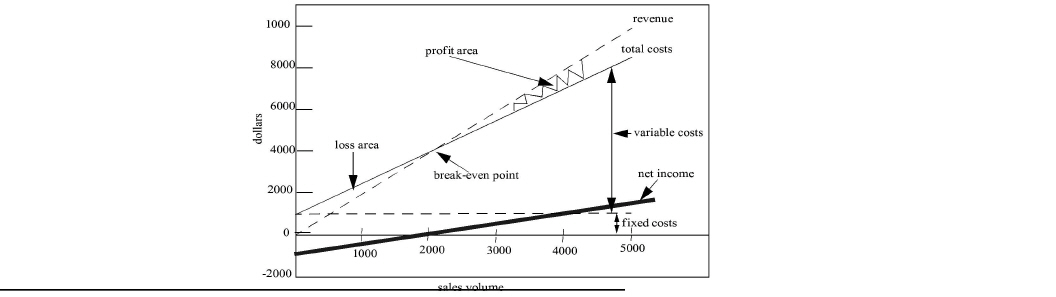
The CVP Chart

The CVP chart is a graphic presentation of the profit equation. Many decision makers prefer graphics instead of numbers because they can “see” a “picture” of the business. Moreover, a chart enables them to understand the relationship of cost, volume, and profit over a range of activity. Quick-Button's CVP chart is displayed in Exhibit 18-2. Carrie considered her relevant range to include sales volumes from zero to 5,000 buttons per year.

Sales volume is plotted on the horizontal axis and dollars on the vertical axis. The loss and profit areas are designated with arrows. To the left of the BEP, Carrie will suffer a loss because total costs are greater than revenues. To the right of the BEP, she will earn a profit because revenues are greater than total costs. In plotting the total costs line, she also included the fixed costs line to differentiate between total fixed and variable costs.

INCREMENTAL CVP ANALYSIS

The contribution margin approach, using the factored form of the profit equation, lends itself to incremen­tal analysis. This type of CVP analysis often addresses “what-if” questions. For example, what if sales volume can be increased by 400 buttons? How much will profits increase? Or, what if Carrie sets a profit goal greater than zero (the BEP)? How many more buttons must she sell to obtain this target profit? This latter question is the second of the three questions Carrie is considering with respect to Quick-Button.

CVP Rules

Before demonstrating how CVP analysis is done incrementally, some mathematical relationships must be understood. These are called “CVP rules.”

1. A dollar change in contribution margin creates the same dollar change in profit (within the relevant range).

2. A unit change in volume multiplied by CMU equals the change in contribution margin.

3. A percentage change in volume multiplied by contribution margin equals the change in contribution margin.

4. A dollar change in revenues multiplied by the CM ratio equals the change in contribution margin. (Cau­tion: This relationship is only true if the change in revenues is caused by a change in volume, not by a change in sales price.)

5. A dollar change in fixed costs creates the opposite change in profit (as fixed costs go up, profit goes down).

6. If there is a change in sales price or variable costs per unit (the elements of CMU), calculate the change in CMU first. Then multiply it by volume to obtain the change in contribution margin.

7. If there are simultaneous changes in one or both elements of CMU and in sales volume, calculate the new contribution margin and compare it to the old contribution margin to obtain the change in contribution margin.

These rules are summarized and demonstrated in Exhibit 18-3.

“What-If” Analysis

“What-if” questions are asked in master budgeting meetings as well as during day-to-day operations of the profit center manager. Using the factored form (the contribution margin approach) of the profit equation and thinking incrementally will allow modern management accountants to answer these questions immedi­ately without returning to their desks for more calculations. Profit center managers are not likely to be pleased when a management accountant says, “I'll have to get back to you later on that.” They need quick and accurate answers within the meeting. To illustrate, consider the following scenario based on the Quick-Button example found on the next page:

Wouldn't it have been better if Carrie had responded, “Let's see. If sales volume increases 300 buttons with a CMU of 50 cents each, then contribution margin will increase $150. This will cover the incremental advertising costs of $100 and leave an extra $50 in profits.” If Carrie had been proficient in incremental CVP analysis, the meeting could have continued without having to be rescheduled sometime in the future!

 

WHAT IF I CAN INCREASE SALES VOLUME? At her meeting with John Enterest, Carrie forecast a sales volume of 2,400 buttons, as shown in Exhibit 18-4. She now knows this is 400 buttons above her BEP. Because of her inability to answer John's question, Carrie realized the need to become more compe­tent in incremental CVP analysis for solving what-if questions. While John was on vacation, Carrie sepa­rated his question into two parts: (1) What is the effect on profits if sales volume increases by 300 buttons? and (2) What is the effect on profits from spending $100 on advertising?

Target sales vol. = (Fixed costs + Profit) - CMU + 300 buttons = (0 + Profit) x $0.50

Solving for the change in profit:

Profit = + 300 buttons x $0.50 = + $150

Alternatively, Carrie can use CVP rule 2:

Volume x CMU = + 300 buttons x $0.50 per button = + $150

If 300 more buttons can be sold, each generating another 50 cents in CMU, then contribution margin will increase by $150. Applying rule 1, a change in contribution margin will yield the same change in profit. This is true only over the relevant range in which total fixed costs do not change if volume changes. Carrie can also solve for the change in profits by using the profit equation approach. The equation, though taking longer to solve, will always work.

Profit = (CMU x Volume) - Fixed costs = ($0.50 per button x 2,700 buttons) - $1,000 per year = $350

Carrie's original base case projection (2,400 buttons per year in Exhibit 18-4) showed a profit of $200. Thus, profit will increase $150 to $350

   

To finish this example, the increase in contribution margin results from an increase in fixed costs (the $100 expenditure for advertising). CVP rule 5 states that a change in fixed costs causes the opposite change in profit. In other words, if fixed costs go up $100, then profit goes down $100. Subtracting the change in fixed costs from the change in contribution margin produces the net $50 increase in profit.

WHAT IF I SET A TARGET PROFIT GOAL? Originally, Carrie also wanted to know, “What sales volume is necessary to realize a target profit?” Assume Carrie sets a profit goal of $200 for 2005. As Exhibit 18-4 shows, she will have to sell 2,400 buttons. She can solve for this incrementally:

Target sales volume = (Fixed costs + Profit) / CMU = (0 + $200) - $0.50 per button = +400 buttons

Carrie will have to sell 400 buttons above the BEP (2,000 buttons). But What if she wants another $300 in profits? If Carrie wants $300 more in profits, regardless of the level of profits she already has, she will have to sell another 600 buttons.

In this illustration, Carrie set an absolute dollar amount of profit. Conceptually, this is just another fixed cost—the payment to the owner. But, what if she stated her profit goal as a percentage of sales revenues? For example, Carrie sets a profit goal of 5 percent of sales. Exhibit 18-5 shows the sales revenues neces­sary to achieve a 5 percent profit. The projected profit of $250 is 5 percent of the $5,000 sales revenues.

In this situation, conceptually speaking, a profit goal stated as a percentage of revenues is just another variable cost. Therefore, profit will not be in the numerator of the profit equation because it is not an abso­lute amount (a fixed cost). Instead, it will now be in the denominator:

Target sales revenues = Fixed costs / (CM ratio - Profit percentage)

   = $1,000 / (25% - 5%)

   = $5,000 per year

Many different types of what-if questions can be asked:

• What if a special order is possible? What is the lowest sales price Carrie can bid?

• What if a firm has an opportunity to buy a part instead of making it? Will buying increase profits?

• What if a part can be sold instead of processed further into a final product?

• Will selling it now increase profits?

• What if a firm does not have enough materials or labor to make all the different types of products it usu­ally sells? Which products should be made?

These kinds of profit management questions are considered in the next chapter. Incremental CVP analysis provides a powerful tool for the management accountant to use in efficiently answering such questions.

Margin of Safety

The third question Carrie originally considered involves the risk of not covering fixed costs (i.e., not breaking even). Measuring this risk involves the calculation of the margin of safety. This is the difference between the sales forecast and the break-even point and can be expressed by the following equation:

Margin of safety =   (Sales forecast - BEP) / Sales forecast

   = (2,400 buttons - 2,000 buttons) / 2,400 buttons

   = l6%⁵

Quick-Button's sales can decrease by 400 buttons, or 16 percent of the sales forecast, before Carrie suffers a loss. If actual sales are below the forecast by more than 16 percent, then Carrie will not break even. These computations can be a useful guide. If the marketing and cost data that Carrie has collected are fairly accurate, then she and John Enterest can consider this a high margin of safety, which indicates low risk. They do not expect that her sales forecast will be off by more than 16 percent. If, on the other hand, her margin of safety was 5 percent, then even a small decline in sales would result in a loss. Consequently, a low margin of safety indicates a high risk of not breaking even.

MULTIPLE PRODUCTS AND INCOME TAX CONSIDERATIONS

The Quick-Button case involved just one product, but many enterprises sell multiple products. Further­more, all profit-making enterprises are subject to income taxes. These extensions to CVP analysis are con­sidered next.

Sales Mix

Sales mix is the relative distribution of sales among the various products sold by a business. Suppose that Tommy Telford is preparing a business plan to launch his venture, New-Wave Designs. He plans to make and market designer caps and T-shirts. Tommy has prepared a projected sales mix for the first fiscal year as follows:

The sales mix for caps and T-shirts can be expressed as relative percentages (as here) or as the ratio of 60 percent to 40 percent (60:40). If this sales mix remains constant over the budget horizon, both the BEP and the sales necessary to achieve a target profit can be calculated using the CVP and break-even equations presented earlier in this chapter.

To illustrate the calculation of the BEP for New-Wave Designs, assume that fixed costs are $24,000. In addition, assume that the unit sales price and variable costs are as follows:

In computing the BEP, each product is considered as a component of an overall New-Wave product called the “package.”⁶ To calculate the BEP, a weighted-average sales price, variable cost per package, and CMU are needed:

The package's variable cost ratio is 70 percent of sales ($2.24 / $3.20), and the CM ratio is 30 percent ($0.96 - $3.20). The overall BEP is computed using the profit equation in its factored format:

BEP = Fixed costs of $24,000 - CMU of $0.96 per package = 25,000 packages

Because the sales mix is 60 percent for caps and 40 percent for T-shirts, the BEP is 15,000 caps (25,000 packages x .60) and 10,000 T-shirts (25,000 packages x .40). The foregoing analysis is summarized in the following contribution margin income statement:   

If Tommy wants to earn a target profit of $20,400:

Target sales volume = (Fixed costs + Profit) / CMU

   = ($24,000 + $20,400) / $0.96

   = 46,250 packages

The sales quota for caps is 27,750 (60 percent of 46,250), and for T-shirts it is 18,500 (40 percent of 46,250). This can also be solved incrementally. The profit goal changes from zero (BEP) to $20,400:

Target sales volume = (Fixed costs + Profit) / CMU

   = ($0 + $20,400)/ $0.96 per package

   = 21,250 packages

Sales volume of caps will have to increase 12,750 (60 percent of 21,250) from the BEP of 15,000 caps to 27,750 caps. Sales volume of T-shirts will have to increase 8,500 (40 percent of 21,250) from its BEP of 10,000 to 18,500 T-shirts.

Income Tax Considerations

If Tommy realizes a profit of $20,400, he will have to pay income taxes and self-employment taxes. Assume these two taxes amount to 40 percent.

 This profit amount is not acceptable to Tommy because he wants $20,400 after taxes. The aftertax profit is 60 percent (1 - Tax rate) of the pretax profit. Solving for the pretax profit needed:

Pretax profit = Aftertax profit - (1 - Tax rate) Substituting this into the profit equation:  = 60,417 packages per year⁷ 

 

What if Tommy's target profit is not an absolute dollar amount, but rather is 5 percent of sales revenues after taxes?

Target sales revenues = Fixed costs / [CM ratio / (Profit percentage / (1 - Tax rate))

= $24,000 / [30% - (5% / (1 -40%))]

= $110,770 per year (rounded up)

SENSITIVITY ANALYSIS AND FINANCIAL PLANNING SOFTWARE

In addition to the preceding analysis, modern profit management also involves sensitivity analysis, which shows how the profit equation responds to changes in the CVP parameters. Sensitivity analysis is a helpful tool for showing the results of different assumptions about the CVP elements. It involves examining the impact of reasonable changes in “base case” assumptions. For example, management accountants might make calculations using several different estimates of variable costs, fixed costs, and sales prices. The effect of these changing parameters on the break-even point can then be studied relative to a most likely scenario.

Essentially, sensitivity analysis is an approach for dealing with uncertain data and other decision risks. Decisions always involve inputs, such as assumptions, estimates, and simplifications, all of which are prone to errors of varying degrees.⁸ Sensitivity analysis can be used to:

• Identify those variables that are most/least sensitive to changes in assumptions.

• Make better profit decisions.

• Decide which data estimates should be refined.

• Focus managerial attention on the most critical elements of a scenario.⁹

This analysis may consider only a few variables, or it may systematically consider all. It may analyze only one variable at a time (known as relative sensitivity), multiple variables, or scenarios of plausible sets of changes. These sensitivities may then be presented through words, tables, or graphs.

Rapid advances in desktop computer technology have removed the barrier of burdensome calculations from sensitivity analysis. Data points are easily obtained through multiple runs of a simple spreadsheet model. Hard-copy output can then be automatically generated to summarize the results. This output usu­ally takes the form of a line graph, bar chart, or break-even graph (CVP chart), all with varying axes and notations.

A sensitivity analysis can be done using any measure, for example, injuries per year, net sales revenue, internal rate of return, present worth, or profit. No matter what form the output takes, it will always show how the chosen measure varies as decision parameters are changed within reasonable limits.

Using Graphical Sensitivities with CVP Analysis

The Quick-Button case can be used to illustrate sensitivity analysis. Based on new sales and cost data and incremental CVP analyses that Carrie Copolla performed for various alternatives, she now estimates the following;

• Sales price per button. $1.30

• Variable cost per button: $0.52

• Fixed costs (one year): $1,560

This will be the base case for her sensitivity analysis. The break-even point is still 2,000 buttons annually.

Carrie has also determined what she considers to be limits of reasonable change for her price and cost data. To be competitive, she feels her button sales price can vary plus or minus 19 percent from her $1.30 esti­mate. Her variable cost estimate could change by as much as 15 percent. Finally, fixed costs could be 10 percent less than estimated, but they could be as much as 30 percent higher. Carrie uses this information with her profit equation to create a spreadsheet generating three tables.

Exhibit 18-6 holds variable cost and fixed costs at their base case values while varying sales price over the 19 percent range. The table also shows the percentage change from the base case for each sales price. The goal of her three tables is to calculate the break-even point under each condition, as shown in the last col­umn.

 

Exhibit 18-7 holds sales price and fixed costs at their base case values while changing the variable cost per unit. Similarly, Exhibit 18-8 varies only the fixed costs over its range.

 

The percentage change from the base case, and the BEP from the three spreadsheet tables are plotted in Exhibit 18-9. Each of the three plots represents the relative sensitivity of the BEP to a particular parame­ter. The plots intersect at the base case. From this graph, Carrie can see that the break-even point, in units sold, for her Quick-Button business is most sensitive to the price she charges for her buttons since that curve has the greatest slope. Therefore, if she wants to decrease the number of units needed to break even, the most effective way to do so is to raise her price. Decreasing either variable or fixed costs is not nearly as effective since these trend lines are flatter.¹⁰ 

A more typical planning and forecasting situation will very likely involve a great many more inputs than just price and costs. In such cases, sensitivity analysis can assist profit managers in making the most effec­tive use of planning resources by allocating them to researching the most critical of the inputs.

Using Graphical Sensitivity Analysis for Decision Making

Sensitivity analysis provides knowledge to managers to help them explore how certain changes may affect a decision. In the accompanying NPV Corporation case (see p. 852), sensitivity analysis gives manage­ment a chance to experiment with different assumptions before making a final decision.

Besides the uncertainty in the demand's growth rate, other base case assumptions can be challenged. For example, the problem horizon (study period) and the discount rate are somewhat arbitrary selections, and the initial cost of microwave installations is often higher than expected. Top management insists that the effects of these uncertainties on the present value of the project be analyzed before a decision is made. The chief variables to be analyzed and their limits of reasonable change are as follows:

Microwave. Initial cost (-40%, +100%), operating costs (-40%, +60%), capacity (-10%, +20%), and life (-40%, +100%).

Leased lines. Cost per line, including amortization of company-supplied interfaces (-20%, +20%), and growth rate of line rates (-80%, +300%).

General. Demand's growth rate (-100%, +50%) and discount rate (-50%, +70%).

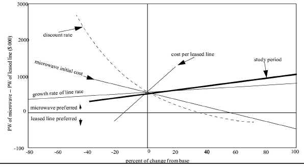
The relative sensitivity of the alternatives' present worth (PW) to each variable is shown in Exhibit 18-10. Note that the vertical axis represents the difference in present worth (PW) between the two alternatives, and the horizontal line at zero is a line of indifference. Above this line, microwave is preferred. Below this line, the leased lines is preferred. Management has already determined a single most likely scenario for the project, and this is taken as the base case. In the exhibit, the base case clearly favors the microwave alter­native because it occurs above the line of indifference.

 

It's important to realize that the natural units for the analyzed variables may be different from each other. For instance, the discount rate is in percent, while the microwave initial cost is in dollars, and the demand's growth rate is in megabits per second per year. For this reason, to readily compare the graphs a common metric must be identified. In Exhibit 18-10, this is the percentage change from the base case, which is shown as the horizontal axis. Of course, lines representing the variables all intersect at the base case point.

Financial Planning Software

Although spreadsheet programs can perform many types of profit planning analyses, financial planning software is often more efficient. It also provides many more sophisticated calculations than can be done with a spreadsheet program, as shown in the Amherst Company case.

BUILDING A WHAT-IF SCREEN. With these data, a what-if screen produced by a financial planning software program¹¹ can be set up to reveal the results of changing conditions. The initial what-if screen and its results are displayed in Exhibit 18-11. At the bottom of the screen are the equations and data used by the program to generate the values at the top of the screen. This initial screen becomes the base case. When a variable receives a new definition (i.e., is changed), this definition replaces the one in the base case. The base case, however, is still stored in memory and can be recalled at any time.

Suppose that management wants to see the results it dollar sales grow by 15 percent rather than 25 percent per period, while variable costs remain the same as in the base case. All the management accountant has to do is change the multiplier to 1.15 instead of 1.25. The results are computed instantly and displayed on the screen as presented in Exhibit 18-12.

 The management accountant can also change several variables, not just one, when creating a what-if screen. For example, the management accountant may want to determine the effect of simultaneous changes in both dollar sales and variable costs:

Sales = 100, Previous x 1.12

Variable costs = 70, Previous + 20

The program will immediately compute new values based on these new variables.

In many what-if analyses, the management accountant may want to change a variable in one or more peri­ods from its value in the base case. The what-if feature can be used for all periods, as in the preceding examples, or for selected periods. To illustrate, if management expects no change in dollar sales for two periods but wants to give new values thereafter:

Sales = Prior 2, Previous x 1.20

The user can also update the base case if new assumptions lead to better results than the initial base case assumptions. In other words, the user has created a new base case against which other what-if cases are to be judged. If desired, the user can keep the initial base case and save the new base case under another name. In this way, both the initial and the updated models are available for use.

USING THE GOAL-SEEK FEATURE. Another powerful feature is goal-seek. Through goal-seek, the program calculates the value a particular variable has to have to achieve a desired level of performance. For example, the management accountant might type the goal as:

Goal: Contribution margin = 25, Previous + 20

This goal states that the contribution margin is to start at $25,000 and to increase by $20,000 each period. Once the goal is established, the program asks for the variable to be adjusted:

Adjust: Variable costs

The program then solves the model and displays the results as shown in Exhibit 18-13.

 The results of the goal-seek screen indicate that variable costs must be reduced to the amounts shown for each period if the company is to realize a contribution margin increase of $20,000 in each period begin­ning with a contribution margin of $25,000 in period 1.

Goal-seek can also be used in just one period, say, period 4. For example, the user might specify:

Goal: Contribution margin [4] = 60 Adjust: Sales [4]

In the base case (Exhibit 18-11), sales of $195,310 in period 4 produce a contribution margin of $45,310. If management can control variable costs at $150,000 and increase sales to $210,000, then the company will achieve a contribution margin of $60,000.

ANALYZING TARGET PROFITS. Assume that the Amherst Company is planning to expand its opera­tions and is considering three alternatives with target profits set at $100,000, $150,000, and $200,000, respectively. To round out the scenario, the management accountant estimates fixed costs at $200,000, $300,000, and $400,000, respectively, for the three alternative expansion plans. The contribution margin (CM) ratio can range from .40 to .60 for each alternative.

Management wants to know the dollar sales level that the enterprise must generate to earn the target prof­its. The program accesses the fixed costs, target profit, and CM ratio at each level, inputs them in the profit equation, and computes the 27 sales revenues shown on the CVP analysis screen in Exhibit 18-14.

Managers can input new values for target profits, fixed costs, and CM ratios to see the effect of changing these variables and to gain a clearer perspective by viewing a wide range of cost, volume, and profit pat­terns. The objective of such analyses is to enhance management's decision-making acumen. The use of spreadsheet programs and financial planning software can contribute to improving profit management, resulting in a high-quality profit management accounting system.

SUMMARY OF LEARNING OBJECTIVES

The major goals of this chapter were to enable you to achieve four learning objectives:

Learning objective 1. Build a profit equation for an enterprise or product line.

The profit equation provides a means of expressing the relationships among variable and fixed costs, sales volume, and their effects on profit. Within a specified relevant range, a linear equation is usually created. It is assumed that sales price and variable costs are constant per unit, fixed costs are constant in total, begin­ning and ending inventory levels do not change, and sales mix is constant when dealing with multiple products.

The profit equation, especially in its factored form, allows the management accountant to quickly and accurately calculate the profit for any level of sales volume within the relevant range. It also promotes incremental analysis by measuring the change in any variable within the equation, given target values for the other variables. The profit equation and its most useful factored forms are summarized in Exhibit 18-15.

Learning objective 2. Use cost-volume-profit (CVP) analysis to analyze different profit-making alternatives.

The break-even point (BEP) is a critical measurement in CVP analysis. It is at this point that total costs equal total sales and the profit is zero. CVP and break-even analysis can be performed by using the equa­tion approach or the contribution margin approach. Regardless of the method used, the results will be the same.

The equation approach is based on the profit equation:

(CMU x Volume) - Fixed costs = Profit

The contribution margin approach is based on the contribution margin, which is sales revenues less vari­able costs. The contribution margin is most useful when stated as contribution margin per unit (CMU) or as a contribution margin (CM) ratio. The contribution margin approach uses the profit equation in one of its factored forms (see Exhibit 18-15).

The following data apply to Pizza King:

• Unit sales price: $10

• Unit variable cost: $6

• Fixed costs: $2,000/period

To calculate the BEP:

BEP = Fixed costs / CMU = (2000 $/_period) / (4 $/_pizza) = 500 pizzas/_period

A contribution margin-based income statement proves this computation:

CMU is the amount that each pizza contributes to covering fixed costs and to profit. If CMU is $4 per unit, each pizza sold will provide $4 to cover fixed costs and contribute to profit. If Pizza King sells 600 pizzas, the first 500 will cover the $2,000 in fixed costs ($4 x 500 pizzas), and the last 100 pizzas will contribute $400 to profit ($4 x 100 pizzas).

The CM ratio is computed as follows:

CM ratio = Sales price $10 = 40%

Using the CM ratio, the break-even revenue (BER) is computed as follows:

BER = $2,000 / .40 = $5,000

If the target profit for Pizza King is $800, then the sales revenue necessary to achieve this target profit is computed as follows:

Revenue goal = ($2,000 + $800) / .40 = $7,000

The sales volume necessary to meet the target profit of $800 is 700 pizzas ($7,000 / $10 sales price per pizza). This can also be computed as follows:

Sales quota = ($2.000 + $800) / $4

= 700 pizzas

Working incrementally, the additional sales volume and revenues needed to generate an additional $800 in profit can be calculated as:

Target sales volume = (Fixed costs + Profit) / CMU

= + $800 - $4 per pizza

= +200 pizzas (above BEP)

Target sales revenues = (Fixed costs + Profit) / CM ratio

= +$800 / 40%

= +$2,000 (above BER)

The margin of safety is the excess of budgeted sales over break-even sales. As a percentage, the margin of safety is computed as follows:

Margin of safety (%) =

= (Budgeted sales - Break-even sales) / (Budgeted sales)

= (700 pizzas - 500 pizzas) /  700 pizzas = 28% (rounded down)

Managers use the margin of safety to evaluate budgeted operations for the forthcoming period or to deter­mine the degree of risk in launching a new business venture. A high margin of safety serves as a cushion and means low risk. A low margin of safety means high risk.

Learning objective 3. Apply CVP formulas to situations involving sales mixes and income taxes.

Sales mix, also termed product mix, is the relative distribution of sales among multiple products. Assume that Sierra Sid sells two products, A and B.

The sales mix is 25 percent product A and 75 percent product B. Product C, which is the overall product, is composed of products A and B. Total fixed costs are $7,400. How many units of each must Sierra Sid sell to break even? The following calculations are used to answer this question:

Weighted-average sales price = ($20.00 x .25) + ($15.00 x .75) = $16.25 per product C

Weighted-average variable costs = ($10.00 x .25) + ($6.00 x .75) = $7.00 per product C

Fixed costs

Product C BEP = FC / CMU

= $7,400 / ($16.25 - $7.00)

= 800 units of product C

Product A BEP = 800 units x .25

= 200 units of product A

Product B BEP = 800 units x .75

= 600 units of product B

Proof of the preceding calculations is illustrated in the following contribution margin income statement:

Assume Sierra Sid sets an after-tax profit goal of $15,000 and anticipates an income tax rate of 20 percent. How many total products (Product C) will have to be sold to obtain this target profit?

Sales quota = [Fixed costs + (Aftertax profit / (1 - Tax rate)] /  CMU

[$7,400 + [$15,000 = (1 - 20%)] / $9.25 = 2,828 total products (rounded up)

Learning objective 4. Describe how computer programs can assist in CVP analysis.

Electronic spreadsheets and various financial planning software packages provide an efficient way for management accountants and managers to work directly with the computer, taking advantage of its com­putational speed and its ability to store massive amounts of data. These software packages provide a sim­ple, natural way of communicating with the computer. Moreover, most of these packages are interactive; they permit the user to sit at the workstation or PC and receive instant feedback. Thus, the user can easily create new CVP models, ask what-if questions, and obtain answers quickly and at a low cost. The results are less drudgery for management accountants and increased quality of decision making in profit manage­ment.

IMPORTANT TERMS

Break-even point (BEP) The sales volume at which revenues equal total costs, and there is zero profit.

Contribution margin Sales revenues minus variable costs. It is the amount that contributes toward cover­ing fixed costs and then toward profits.

Contribution margin approach A method of CVP analysis that focuses on the contribution margin, using the profit equation in one of its factored forms.

Contribution margin-based income statement An income statement format in which total variable costs are subtracted from sales revenues, creating the contribution margin subtotal, from which fixed costs are then subtracted to yield net income. It differs from a traditional financial accounting for­mat in that costs are organized by behavior rather than by function.

Contribution margin per unit (CMU) Sales price minus variable costs per unit. It is the incremental money available from selling one more product that is used to cover fixed costs and contribute to profits.

Contribution margin ratio (CM ratio) The contribution margin per unit expressed as a percentage of the selling price.

Cost-volume-profit (CVP) analysis The determination and study of the relation-ships among cost, vol­ume or level of activity, and profit. CVP analysis involves the creation and use of the profit equa­tion.

Equation approach A CVP analysis method that uses the profit equation in its unfactored format: (CMU x Volume) - Fixed costs = Profit.

Margin of safety The sales volume in excess of the break-even point. It is usually expressed as a percent­age of the sales forecast and is used as a measure of break-even riskiness.

Profit equation Usually, a linear equation used to summarize CVP relationships. It is: (CMU x Volume) - Fixed costs = Profit.

Sales mix The relative combination in which an organization's products are sold. Sales mix is calculated by expressing the sales of each product as a percentage of total sales.

Sensitivity analysis A type of profit management analysis, usually using software programs, that mea­sures the riskiness of the amounts used in the profit equation. It shows how profit and volume change as other amounts change by certain percentages or absolute amounts.

Variable cost ratio The percentage relationship between variable costs and sales revenues.

DEMONSTRATION PROBLEMS

DEMONSTRATION PROBLEM 1 Break-even calculations.

Quickround manufactures golf carts. The following data pertain to this product:

a. Compute the BEP and BER using the equation approach.

b. Compute the BEP and BER using the contribution margin approach.

c. The expected (or budgeted) sales for the next period are 300 golf carts. Compute the margin of safety.

SOLUTION TO DEMONSTRATION PROBLEM 1

a.

(CMU x Volume) - Fixed costs = Profit

($500 per cart x Volume) - $100,000 = $0

BEP = 200 golf carts

BER can be calculated by multiplying BEP by the sales price:

 BER = 200 golf carts x $800 per cart = $160,000

b. The contribution margin approach simply uses the profit equation in one of its factored forms. To calcu­late how many units must be sold to break even, total fixed cost is divided by CMU:

BEP = Fixed costs / CMU

= $100,000/ ($800-$300)

$100,000 / $500

= 200 golf carts

BER = Fixed costs / CM ratio

= $100,000 / (($800 - $300) / $800)

$100,000 / .625

= $160,0 00

c. Margin of safety = Sales forecast - BEP  / Sales forecast

= (300 carts - 200 carts) / 300 carts = 33.33%

DEMONSTRATION PROBLEM 2 Sales mix.

Landscape Products is a two-product company making square-pointed shovels and yard rakes. The follow­ing budget is developed for the next period:

Note: Total sales in units are made up of 70% shovels and 30% rakes.

Required: Compute the BEP for both products

SOLUTION TO DEMONSTRATION PROBLEM 2.

  

BEP = Fixed costs of $106,500 / $7.10

= 15,000 units

BEP (shovels) = 15,000 units x .70 = 10,500 shovels

BEP (rakes) = 15,000 units x .30 = 4,500 rakes

Assuming that the sales mix will not change, Landscape must sell 10,500 shovels and 4,500 rakes next period to break even.

DEMONSTRATION PROBLEM 3 Break-even calculation considering income taxes.

Gladstone Company's projected data are as follows:

Required: How many units will Gladstone have to sell to earn $30,000 in net income after taxes?

SOLUTION TO DEMONSTRATION PROBLEM 3

Unit sales = Fixed costs + [Target profit (1 - Tax rate)] / CMU

= $60,000 + [$30,000 - (1 - .40)] / $40

= 2,750 units

REVIEW QUESTIONS

18.1 List and briefly define the elements involved in cost-volume-profit (CVP) analysis.

18.2 What are the two goals (purposes) of a profit equation?

18.3 Why is the master budgeting process iterative?

18.4 What is the role of CVP analysis in the master budgeting process?

18.5 How can CVP analysis help profit center managers in their operational control role?

18.6 What are the three basic CVP assumptions?

18.7 Which assumptions also apply to cost equations?

18.8 What is the relationship between a cost equation and a profit equation?

18.9 How are sales revenues and sales prices related?

18.10 What is the independent variable in the profit equation? Why is it the same as in the manufacturing cost equation?

18.11 Define contribution margin and contribution margin per unit. How are they related?

18.12 Write out the profit equation used in the equation approach to CVP analysis.

18.13 Define the break-even point.

18.14 Describe and distinguish between the equation approach and the contribution margin approach.

18.15 How can the profit equation be written as a function of revenues?

18.16 What is the format for the contribution margin-based income statement? How does it differ from the traditional format used in financial reporting?

18.17 Why are fixed costs and profit included only in the totals column and not expressed on a per-unit basis?

18.18 What is the purpose of expressing contribution margin on a per-unit and a percentage basis?

18.19 Compare and contrast the variable cost ratio and the contribution margin ratio.

18.20 How is the CM ratio useful in multiple product CVP analysis?

18.21 Interpret how CMU and fixed costs are related in break-even analysis.

18.22 What is a CVP chart?

18.23 How is incremental CVP analysis useful in profit management decisions?

18.24 Using the data in Exhibit 18-1, make up simple numeric examples to illustrate each of the CVP rules for incremental analysis.

18.25 Describe “what-if” analysis.

18.26 Why can a profit goal, stated as an absolute dollar amount, be considered as just another fixed cost of the business?

18.27 How does the profit equation change if the profit goal is stated as a variable amount?

18.28 Define, illustrate, and interpret the margin of safety.

 18.29 Define sales mix.

18.30 How is aftertax profit related to pretax profit, and how is the profit equation modified to account for an aftertax target profit?

18.31 Define sensitivity analysis.

18.32 What is goal-seek analysis?

18.33 Explain how financial planning software can be useful in CVP analysis.

CHAPTER-SPECIFIC PROBLEMS

These problems require responses based directly on concepts and techniques presented in the text.

18.34 Break-even analysis. The estimates made for Glaxot Company, a one-product company, are as fol­lows:   

Total selling and administrative expenses   <3,100>

Net income before income taxes   $ 2,500

Required:

a. How many units of the product must Glaxot sell to break even?

b. What would be the net income before income taxes if projected unit sales increased by 25%?

c. What would dollar sales be at the BEP if fixed overhead increased by $1,700? [AICPA adapted]

18.35 Multiple choice, income taxes. [CMA adapted] The following statement of income for Davann Company represents the operating results for the fiscal year just ended. Davann had sales of 1,800 tons during the current year. The manufacturing capacity of Davann's facilities is 3,000 tons.

Required: choose the best answer. Each item is independent of every other item.

a. The break-even volume in tons for 2005 is (1) 420 tons, (2) 1,100 tons, (3) 495 tons, (4) 550 tons, (5) some other amount.

b. If the sales volume is estimated to be 2,100 tons in the next year, and if prices and costs stay at the same levels and amounts next year, Davann can expect aftertax net income of (1) $135,000, (2) $110,250, (3) $283,500, (4) $184,500, (5) some other amount.

c. Davann plans to market its product in a new territory. Davann estimates that an advertising and promo­tion program costing $61,500 annually would need to be undertaken for the next two or three years. In addition, a $25 per ton sales commission over and above the current commission would be required for the sales force in the new territory. How many tons would have to be sold in the new territory to maintain Davann's current aftertax income of $94,500? (1) 307.5 tons, (2) 1,095.0 tons, (3) 273.333 tons, (4) 1,545.0 tons, (5) some other amount.

d. Davann is considering replacing a highly labor-intensive process with an automatic machine. This would result in an increase of $58,500 annually in manufacturing fixed costs. The variable manu­facturing costs would decrease $25 per ton. The new break-even volume in tons would be (1) 990 tons, (2) 1,224 tons, (3) 1,854 tons, (4) 612 tons, (5) some other amount.

e. Ignore the facts presented in Requirement (d) and now assume that Davann estimates that the per-ton selling price would decline 10% next year. Variable costs would increase $40 per ton, and the fixed costs would not change. What sales volume in dollars would be required to earn an aftertax net income of $94,500 next year? (1) $1,140,000, (2) $825,000, (3) $1,500,000, (4) $1,350,000, (5) some other amount.

18.36 CVP analysis. The Stillson Company makes a single product. It sold 40,000 units last year with the following results:

 

Stillson plans to improve its product by replacing a component that has a cost of $3 per unit with a new and better component costing $5 per unit in the coming year. A new machine will also be needed to increase plant capacity. The machine will cost $20,000 with a useful life of 5 years and no salvage value. The company uses straightline depreciation on all plant assets.

Required:

a. What was Stillson's BEP in unit sales last year?

b. How many units would Stillson have had to sell in the last year to earn $180,000 in net income after income taxes?

c. If Stillson holds the sales price constant and makes the component change, how many units must be sold in the coming year to break even?

d. If Stillson holds the sales price constant and makes the suggested changes, how many units will the company have to sell to make the same net income as it made after income taxes last year?

e. If Stillson wishes to maintain the same CM ratio, what selling price per unit must it charge next year to cover the increased component costs?

18.37 CVP analysis. Printrite is a retailer for print modules. The projected aftertax net income for the cur­rent year is $600,000 based on a sales volume of 400,000 print modules. Printrite has been selling the print modules at $32 each. The variable costs consist of the $20 per unit purchase price charged by the vendor and a handling cost of $4 per module. Printrite's annual fixed costs are $2,200,000. Printrite's income tax rate is 40%. Management expects that the unit purchase price of the print modules will increase 30%.

Required:

a. What is Printrite's BEP for the current year in unit sales?

b. What would be the aftertax income for the current year with an increase of 10% in sales volume?

c. What will the dollar sales have to be in the coming year to maintain the same aftertax net income as pro­jected for the current year if unit selling price remains at $32?

d. In order to cover a 30% increase in the print module's purchase price for the coming year and still main­tain the current CM ratio, what must the selling price be for the coming year?

 18.38 Break-even analysis for a two-product company. Tranco manufactures two products, Gizmo and Widget. The following are projections for the coming year:

 

a. What is the BEP for Gizmos, assuming the facilities are not used jointly?

b. What is the BER for Widgets, assuming the facilities are not used jointly?

c. What is the composite CMU, assuming that consumers purchase composite units of four Gizmos and three Widgets?

d. If consumers purchase composite units of four Gizmos and three Widgets, what is the BEP?

e. If a composite unit is defined as one Gizmo and one Widget, what is the composite CM ratio?

f. If Gizmos and Widgets become one-to-one complements and there is no change in Tranco's cost func­tion, what is the BER?

18.39 Margin of safety in dollar sales. The Stackrite Company makes printer attachments. The company budgets a margin of safety of 20% for 19X4. Fixed costs are budgeted at $240,000 annually. Variable costs are $6 per attachment. The sales price per attachment is $12.

Required. Compute the margin of safety in dollar sales.

THINK-TANK PROBLEMS

Although these problems are based on chapter material, reading extra material, reviewing previous chap­ters, and using creativity may be required to develop workable solutions.

18.40 Break-even analysis. [AICPA adapted] All-Day Candy Company is a wholesale distributor of candy. The company services grocery, convenience, and drug stores in a large metropolitan area. All-Day has achieved small but steady growth in sales over the past few years while candy prices have been increasing. The company is formulating its plans for the coming fiscal year. Following are the data used to project the current year's aftertax net income of $110,400.

 Manufacturers of candy have announced that they will increase prices of their products an average of 15% in the coming year due to increases in raw materials (sugar, cocoa, peanuts, and so on) and labor costs. All-Day Candy Company expects that all other costs will remain at the same rates or levels as the current year.

Required:

a. What is All-Day Candy Company's BEP in boxes of candy for the current year?

b. What selling price per box must All-Day Candy Company charge to cover the 15% increase in the cost of candy and still maintain the current CM ratio?

c. What volume of sales in dollars must the All-Day Candy Company achieve in the coming year to main­tain the same net income after taxes as projected for the current year if the selling price of candy remains at $4 per box and the cost of candy increases 15%?

18.41 Change in sales mix and income taxes. [CMA adapted]   Hewtex Electronics manufactures two products-tape recorders and electronic calculators-and sells them nationally to wholesalers and retailers. The Hewtex management is very pleased with the company's performance for the current fiscal year. Pro­jected sales through December 31,19X7, indicate that 70,000 tape recorders and 140,000 electronic calcu­lators will be sold this year. The projected earnings statement follows:

It shows that Hewtex will exceed its earnings goal of 9% on sales after income taxes.

The tape recorder business has been fairly stable the last few years, and the company does not intend to change the tape recorder price. Competition among manufacturers of electronic calculators has been increasing, however. Hewtex's calculators have been very popular with consumers. In order to sustain this interest in their calculators and to meet the price reductions expected from competitors, management has decided to reduce the wholesale price of its calculator from $22.50 to $20.00 per unit effective January 1, 19X8. At the same time, the company plans to spend an additional $57,000 on advertising during fiscal year 19X8. As a consequence of these actions, management estimates that 80% of its total revenue will be derived from calculator sales compared to 75% in 19X7. As in prior years, the sales mix is assumed to be the same at all volume levels.

The total fixed overhead costs will not change in 19X8, nor will the variable overhead cost rates (applied on a direct labor hour base). However, the cost of materials and direct labor is expected to change. The cost of solid-state electronic components will be cheaper in 19X8. Hewtex estimates that material costs will drop 10% for the tape recorders and 20% for the calculators in 19X8. Direct labor costs for both prod­ucts will increase 10% in the coming year, however.

Required:

a. How many tape recorder and electronic calculator units did Hewtex Electronics have to sell in 19X7 to break even?

b. What volume of sales is required if Hewtex Electronics is to earn a profit in

19X8 equal to 9% on sales after income taxes?

c. How many tape recorder and electronic calculator units will Hewtex have to

sell in 19X8 to break even?

 18.42 CVP relationships and income taxes. [CMA adapted] R. A. Ro and Company, maker of quality handmade pipes, has experienced a steady growth in sales for the past five years. However, increased com­petition has led Mr. Ro, the president, to believe that an aggressive advertising campaign will be necessary next year to maintain the company's present growth.

To prepare for next year's advertising campaign, the company's accountant has prepared and presented Mr. Ro with the following data for the current year, 19X7:

  

Mr. Ro has set the sales target for 19X8 at a level of $550,000 (or 22,000 pipes).

Required:

a. What is the projected aftertax net income for 19X7?

b. What is the BEP in units for 19X7?

c. Mr. Ro believes an additional selling expense of $11,250 for advertising in 19X8, with all other costs remaining constant, will be necessary to attain the sales target. What will be the aftertax net income for 19X8 if the additional $11,250 is spent?

d. What will be the BEP in dollar sales for 19X8 if the additional $11,250 is spent for advertising?

e. If the additional $11,250 is spent for advertising in 19X8, what is the required sales level in dollar sales to equal 19X7's aftertax net income?

f. At a sales level of 22,000 units, what is the maximum amount that can be spent on advertising if an after­tax net income of $60,000 is desired?

18.43 Break-even analysis with step fixed costs.[AICPA adapted]   Sierra Hospital operates a general hos­pital that rents space and beds to separate departments such as pediatrics, maternity, and surgery. Sierra Hospital charges each separate department for common services to its patients, such as meals and laundry, and for administrative services, such as billing and collections. Space and bed rentals are fixed for the year.

For the year ended June 30, 19 the Pediatrics Department at Sierra Hospital charged its patients an average of $65 per day, had a capacity of 60 beds, operated 24 hours per day for 365 days, and had total revenue of $1,138,800.

Expenses charged by the hospital to the Pediatrics Department for the year were as follows:

The only personnel directly employed by the Pediatrics Department are supervising nurses, nurses, and aides. The hospital has minimum personnel requirements based on total annual patient-days. Hospital requirements, beginning at the minimum expected level of operation, follow:

These staffing levels represent full-time equivalents, and it should be assumed that the Pediatrics Depart­ment always employs only the minimum number of required full-time equivalent personnel.

Annual salaries for each class of employee are as follows: supervising nurses, $18,000; nurses, $13,000; and aides, $5,000. Salary expense for the year ended June 30, 19X7, was $72,000, $169,000, and $110,000 for supervising nurses, nurses, and aides, respectively.

Required: a. Compute the following:

1. The number of patient-days in the Pediatrics Department for the year ended June 30, 19X7. (Each day a patient is in the hospital is known as a “patient-day.”)

2. The variable cost per patient-day for the year ended June 30, 19X7.

3. The total fixed costs, including both allocated fixed costs and personnel costs, in the Pediatrics Depart­ment for each level of operations shown above (i.e., total fixed costs at the 10,000-14,000 patient-day level of operation, total fixed costs at the 14,001-17,000 patient-day level of opera­tion, and so forth).

b. Using the data computed in Requirement (a) and using any other data as needed, compute the minimum number of patient-days required for the Pediatrics Department to break even. You may assume that vari­able and fixed cost behavior and revenue per patient-day will remain unchanged in the future.

c. Determine the minimum number of patient-days required for the Pediatrics Department to earn an annual profit of $80,000.

18.44 Break-even analysis and target profits. Starling Company is a small but growing manufacturer of telecommunications equipment. The company has no sales force of its own; instead, it relies completely on independent sales agents to market its products. These agents are paid a commission of 15% of selling price for all items sold.

Li Kim, Starling's controller, has just prepared the company's budgeted income statement for next year. The statement follows:

   

As Li handed the statement to Tom Remski, Starling's president, she commented, “I went ahead and used the agents' 15% commission rate in completing these statements, but we've just learned that they refuse to handle our products next year unless we increase the commission rate to 20%.”

“That's the last straw,” replied Tom angrily, “Those agents have been demanding more and more, and this time they've gone too far. How can they possibly defend a 20% commission rate?”

“They claim that after paying for advertising, travel, and the other costs of promotion, there's nothing left over for profit,” replied Li.

“I say it's just plain robbery,” retorted Tom. “And I also say it's time we dumped those people and got our own sales force. Can you get your people to work up some cost figures for us to look at?”

“We've already worked them up,” said Li. “Several companies we know about pay a 7.5% commission to their own salespeople, along with a small salary. Of course, we would have to handle all promotion costs, too. We figure our fixed costs would increase by $2,400,000 per year, but that would be more than offset by the $3,200,000 (20 % x $16,000,000) that we would avoid on agents' commissions.”

The breakdown of the $2,400,000 cost figure follows:

“Super,” replied Tom. “And I note that the $2,400,000 is just what we're paying the agents under the old 15% commission rate.”

“It's even better than that,” explained Li. “We can actually save $75,000 a year, because that's what we're having to pay the auditing firm now to check out the agents' reports. So our overall administrative costs would be less.”

“Pull all of these numbers together and we'll show them to the executive committee tomorrow,” said Tom. “With the approval of the committee, we can move on the matter immediately.”

Required:

a. Compute Starling Company's BEP in sales dollars for 19X6, assuming: 1. That the agents' commission rate remains unchanged at 15%. 2. That the agents' commission rate is increased to 20%. 3. That the com­pany employs its own sales force.

b. Assume that Starling Company decides to continue selling through agents and pays the 20% commis­sion rate. Determine the volume of sales that would be required to generate the same net income as in the budgeted income statement for 19X6.

c. Determine the volume of sales at which net income would be equal regardless of whether Starling Com­pany sells through agents (at a 20% commission rate) or employs its own sales force.

d. Based on the data in Requirements (a) through (c), make a recommendation as to whether the company should continue to use sales agents (at a 20% commission rate) or employ its own sales force. Give reasons for your answer. [CMA adapted]

18.45 Break-even analysis and target profits. [CMA adapted] RayLok, Inc., has invented a secret process to measure light intensity and manufactures a variety of products related to this process. Each product is independent of the others and is treated as a separate profit-loss division. Product (division) managers have a great deal of freedom to manage their divisions as they think best. Failure to produce target division profit is dealt with severely, but rewards for exceeding one's profit objective are lavish.

The DimLok Division sells an add-on automotive accessory that automatically dims a vehicle's headlights by sensing a certain intensity of light coming from a specific direction. DimLok has had a new manager in each of the three previous years because the predecessor manager failed to reach RayLok's target profit. Don Barnes has just been promoted to manager and is studying ways to meet the current target profit for DimLok.

The two profit targets for DimLok for the coming year are $800,000 plus an additional profit of $20 for each DimLok unit sold. Other constraints on division operations follow:

• Production cannot exceed sales since RayLok's corporate advertising program stresses completely new product models each year, even though the “newness” of the models may be only cosmetic.

• The DimLok selling price may not vary above the current selling price of $200 per unit but may vary as much as 10% below $200.

• A division manager may elect to expand fixed production or selling facilities; however, the target objec­tive that is related to fixed costs is increased by 20% of the cost of such expansion. Furthermore, a man­ager may not expand fixed facilities by more than 30% of existing fixed cost levels without approval from the board of directors.

Barnes is now examining data gathered by his staff to determine if DimLok can achieve its target profits of $800,000 and $20 per unit. A summary of these reports shows the following:

• Last year's sales were 40,000 units at $200 per unit.

• The present capacity of DimLok's manufacturing facility is 40,000 units per year, but capacity can be increased to 80,000 units per year by an increase in annual fixed costs of $1,000,000.

• Present variable costs amount to $80 per unit, but if commitments are made for more than 60,000 units, DimLok's vendors are willing to offer raw material discounts amounting to $20 per unit, beginning with unit number 60,001.

• Sales can be increased up to 100,000 units per year by committing large blocks of product to institutional buyers at a discounted unit price of $180. However, this discount would apply only to sales in excess of 40,000 units per year.

Barnes believes that these projections are reliable, and he is now trying to determine what DimLok must do to meet the profit objectives assigned by Ray-Lok's board of directors.

Required:

a. Calculate the dollar value of DimLok's present annual fixed costs.

b. Determine the number of units that DimLok must sell in order to achieve

both profit objectives. Be sure to consider all constraints in determining your answer.

c. Without prejudice to your answer in Requirement (b), assume Don Barnes decides to sell 40,000 units at $200 per unit and 24,000 units at $180 per unit. Prepare a pro forma (i.e., forecasted) income statement for DimLok showing whether or not Don Barnes' decision will achieve DimLok's profit objectives.

 18.46 Break-even analysis and optimal production plan. [CMA adapted] The PTO Division of the Galva Manufacturing Company produces power take-off units for the farm equipment business. The PTO Divi­sion, headquartered in Peoria, has a newly renovated, automated plant in Peoria and an older, less auto­mated plant in Moline. Both plants produce the same power take-off units for farm tractors that are sold to most domestic and foreign tractor manufacturers.

The PTO Division expects to produce and sell 192,000 power take-off units during the coming year. The division production manager has the following data available regarding the unit costs, unit prices, and pro­duction capacities for the two plants:

• All fixed costs are based on a normal year of 240 working days. When the number of working days exceeds 240, variable manufacturing costs increase by $3 per unit in Peoria and $8 per unit in Moline. Capacity for each plant is 300 working days.

• Galva Manufacturing charges each of its plants a per-unit fee for administrative services such as payroll, general accounting, and purchasing, as Galva considers these services to be a function of the work per­formed at the plants. For each of the plants at Peoria and Moline, the fee is $6.50 and represents the vari­able portion of general and administrative expense.

Wishing to maximize the higher unit profit at Moline, PTO's production manager has decided to manufac­ture 96,000 units at each plant. This production plan results in Moline operating at capacity and Peoria operating at its normal volume. Galva's corporate controller is not happy with this plan as he does not believe it represents optimal usage of PTO's plants.

Required:

a. Determine the annual break-even units for each of PTO's plants.

b. Calculate the operating income that would result from the division production manager's plan to produce 96,000 units at each plant.

c. Determine the optimal production plan to produce the 192,000 units at PTO's plants in Peoria and Moline, and calculate the resulting operating income for the PTO Division. Be sure to support the plan with appropriate calculations.

18.47 Segmented contribution and CVP analysis. Kalifo Company manufactures a line of electric garden tools that are sold in general hardware stores. The company's controller, Sylvia Harlow, has just received the sales forecast for the coming year for Kalifo's three products: weeders, hedge clippers, and leaf blow­ers. Kalifo has experienced considerable variations in sales volumes and variable costs over the past two years, and Harlow believes the forecast should be carefully evaluated from a CVP viewpoint. The prelimi­nary budget information for 19X8 is presented as follows:

For 19X8, Kalifo's fixed factory overhead is budgeted at $2,000,000, and the company's fixed selling and administrative expenses are forecasted to be $600,000. Kalifo has an effective tax rate of 40%.

Required:

a. Determine Kalifo Company's budgeted net income for 19X8,

b. Assuming the sales mix remains as budgeted, determine how many units of each product Kalifo Com­pany must sell in order to break even in 19X8.

c. Determine the total dollar sales Kalifo Company must sell in 19X8 in order to earn an aftertax net income of $450,000.

d. After preparing the original estimates, Kalifo Company determined that its variable manufacturing cost of leaf blowers would increase 20% and the variable selling cost of hedge clippers could be expected to increase $1 per unit. However, Kalifo has decided not to change the selling price of either product. In addition, Kalifo has learned that its leaf blower has been perceived as the best value on the market, and it can expect to sell three times as many leaf blowers as any other prod­uct. Under these circumstances, determine how many units of each product Kalifo Company would have to sell in order to break even in 19X8.

e. Explain the limitations of CVP analysis that Sylvia Harlow should consider when evaluating Kalifo Company's 19X8 budget. [CMA adapted]