Chapter 13  :  Cost Management For Logistics

LEARNING OBJECTIVES

Learning objective 1. Discuss how and EDI or other web-based payment system can support logistics and reduce costs.

Learning objective 2. Define procurement, and explain how procurement costs can be reduced.

Learning objective 3. Describe the transportation activity, and examine how productivity of this activity can be increased.

Learning objective 4. Explain how to manage inventory costs.

Learning objective 5. Describe the warehousing activity, and explore ways to manage warehouse costs.

INTRODUCTION

Just as management accountants, production people, and engineering personnel join forces in developing methods of costing products and services and managing production costs, so must management accoun­tants and logistics personnel work together to manage logistics costs. The potential payoff of effective cost management for logistics is substantial, because logistics costs account for between 20 and 50 percent of total costs in most companies. Often, logistics costs exceed production costs.

Logistics systems consist of the integration of procurement, transportation, inventory management, and warehouse activities to provide the most cost-effective means of meeting internal and external customer requirements. Logistics costs are expenditures incurred for planning, implementing, controlling, and operating all logistics activities.¹ This chapter is intended to assist management accountants in improving identification, measurement, and management of logistics costs.

USING ELECTRONIC DATA INTERCHANGE IN THE LOGISTICS SYSTEM

Electronic data interchange (EDI) was described in Chapter 3 as a set of standards and information tech­nology that enable purchase orders, invoices, and payments, to be transferred electronically between par­ticipating companies. Many companies and industries are moving toward implementation of EDI technology. Besides interconnecting companies with suppliers, customers, and common carriers, EDI sys­tems are used by commercial banks to handle electronic financial transactions (e.g., paying suppliers and common carriers and collecting from customers).

LEARNING OBJECTIVE 1

 Discuss how an electronic data interchange (EDI) system can support logistics and reduce costs.

Improving Performance and Gaining Cost Savings with EDI

A customer order triggers the logistics system. The ability to capture all pertinent data immediately and ensure their timely flow to all users has direct impact on the effectiveness and efficiency of the entire logis­tics system. Mishandled customer orders and slow or erratic flow of information can lead to lost customers and excessive procurement, transportation, inventory, and warehousing costs, as well as disruptions in the production process. EDI provides the foundation for the logistics system and offers significant potential for improving logistics performance and increasing profits.

Significant cost savings can be realized with a fully integrated EDI system compared to nonelectronic communications. For example, Service Merchandise, Inc., a major catalogue discount retailer, has been able to cut the cost of a single purchase order transaction from $50 to $15 using EDI.² This cost savings is due to:

• Reduced errors

• Reduced paperwork

• Increased order processing speed, which decreases costs throughout the logistics system

Designing an EDI System

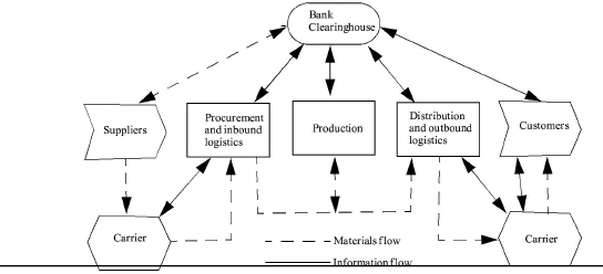
The management accountant at Moparts, Inc., has proposed an EDI system to replace the company's pres­ent paper-based logistics systems. A commercial bank will be connected to the EDI technology to serve as a financial clearinghouse. The new EDI system design is illustrated in Exhibit 13-1

.

Key Elements of the EDI System

Chapter 3 described the EDI system from the viewpoint of computers and telecommunications. The EDI system also requires other key elements to make it workable for an organization, including the following:

 

• Bar codes, QR codes, RFID tags, etc.

• Customer order model

• Picking and packing lists

• Portable terminals

• Flash reports

• Inventory control models

Bar Codes. All items in inventories use bar codes for identification and for product movement on comput­erized conveyor belts. As an item moves along the conveyor belt, it is scanned automatically, identified, and routed to the correct spur of the conveyor where it will be unloaded for production, loaded for ship­ment, or placed in a warehouse. All pertinent data relating to the item and its movement are also fed into the EDT system for producing various management reports, such as the order activity report in Exhibit 13-2.

CUSTOMER ORDER MODEL. To make an EDI system functional, a number of software modules must be utilized. Structured English or pseudocode is used in designing these software modules. For example, Exhibit 13-3

 illustrates a module of the customer order model designed in structured English. Other modules that check credit, process backorders, and so forth are designed in a similar manner. Once the design has been approved, it is automatically programmed in a computer language (e.g., COBOL or C) and integrated into the system using computer-aided software engineering (CASE) tools. All the inte­grated software modules that drive the customer order model automatically perform procedures necessary to service a customer order and run the EDI system.

AUTOMATICALLY GENERATING PICKING AND PACKING LISTS.

All customer orders automatically generate a picking and packing list, such as the list in Exhibit 13-4. The picking and packing list tells pickers in the warehouse which items have been ordered and must be picked, where they can be picked, and the most efficient sequence in which they should be picked. Bar codes are automatically prepared and attached to the picking and packing list.

Pickers retrieve ordered products, affix the proper shipping bar codes, and send the products down a con­veyor belt in trays to a laser scanner. The laser scanner reads the bar codes, determines which order an item belongs to, and tips its tray down the appropriate packing chute.

At the bottom of the chute, packers, who also have a copy of the picking and packing list, assemble orders and pack them in boxes for shipping. Packers affix a second bar code to the outside of each box, and a sec­ond laser scanner ensures that each box is routed to the appropriate loading dock for shipment via a spe­cific common carrier or company truck. At this point, the central EDI computer takes over and begins to prepare EDI data, such as bills of lading, shipment notices, and invoices. Also, all pertinent records in the database are updated automatically.

USING PORTABLE TERMINALS. Inventory counting and verification are handled by computer termi­nals hung from workers' belts. A laser-wand attachment is used to read the product identification bar code of every item in inventory. These data are then transmitted to the central EDI computer for update of the inventory database.

Every salesperson in the field has a laptop computer, which also has access to the EDI system. These lap­tops are used for electronic mail and paging as well as for facilitating a sale to a customer. The salesperson, sitting in a customer's office, can access a variety of models ranging from engineering specifications and design aids to economic analyses. Upon making a sale, the salesperson immediately transmits the sales data to the system to begin customer order processing.

USING FLASH REPORTS. Flash reports are generated automatically by the EDI system and displayed on terminal screens at strategic points throughout the company. Examples of flash reports include receiv­ing orders, shipping orders, and rejected customer orders. Generally, flash reports require immediate action by some designated worker or manager. For example, warehouse workers receive a flash report notifying them what products will arrive, when, and by which carrier.

INVENTORY CONTROL MODELS. Inventory control models, like the customer order model, must be integrated into the EDI system. Inventory control deals with when to order or produce items and how much to order or produce. The when-to-order-or-produce question is answered by reorder points pro­grammed into the system. The system monitors the depletion of inventory and automatically initiates an order to replenish the inventory when the reorder point is reached or exceeded. The how-much-to-order-or-produce question is usually answered by a mathematical model. These inventory control models, referred to as economic order quantity (EOQ) or economic batch quantity (EBQ) models, are described later in this chapter.

Other methods of controlling inventory are just-in-time (JIT) coupled with a kanban system, as described in Chapter 2. Material requirements planning (MRP) and manufacturing resource planning (MRP II) are software packages that can also be incorporated into EDI systems to aid inventory management, as described in Chapter 3.

MANAGING PROCUREMENT COSTS

LEARNING OBJECTIVE 2

Procurement includes the purchasing function and verification of inbound raw materials or products at the receiving dock. This logistics activity has the following goals:

• Select and evaluate suppliers (covered in Chapter 11)

• Provide an uninterrupted flow of materials and services to operate the enterprise

• Minimize inventory costs

• Acquire materials and services at the lowest cost and at the quality that best meets the company's needs

• Operate the procurement activity at the lowest possible cost

• Ensure that the correct product is received in the correct quantity and with acceptable quality

Managing the Procurement Activity

In addition to careful evaluation and selection of suppliers, the procurement activity itself should be man­aged properly. The following are selected performance measurements that will help accomplish this:

Purchase orders per buyer per week = # of POs per week / # of buyers

   = 400 POs / 20 buyers = 20 POs/buyer/week

Administrative cost per PO =  Administrative cost per week / # of POs per week

   = $8000 / 400 POs = $20/PO

Service to production = # of complaints from production per week / # of orders released to production per    week

   = 4 complaints from production / 100 orders released to production

   = 4% of orders released to production received complaints

Relationship of Just-in-Time to Procurement

The most effective approach to managing the costs of the procurement activity is to reduce the need for this activity. JIT procurement achieves this goal by developing long-term relationships with a few certified suppliers.

The characteristics of the JIT procurement activity are interrelated. They are grouped in Exhibit 13-5

 under three general categories: suppliers, quantities, and quality.

WHAT ARE THE BUYER BENEFITS OF JIT PROCUREMENT? Exhibit 13-6

 summarizes the benefits of JIT procurement to the buyer. All the benefits result in substantial cost savings for the buying company.

WHAT ARE THE SUPPLIER BENEFITS OF JIT PROCUREMENT? Exhibit 13-7

 summarizes the certified supplier benefits of JIT procurement. The certified supplier or vendor receives a long-term pur­chase agreement from the buyer. This provides the supplier with the opportunity to reduce nonvalue-added activities, reduce capacity and resources, retain a trained labor force, reduce inventories, and implement JIT procurement systems with its own suppliers.³

MANAGING TRANSPORTATION COSTS

LEARNING OBJECTIVE 3

Transportation involves the movement of products (raw materials, parts, supplies, subassemblies, work-in-process, finished goods) from point-of-origin to point-of-consumption. Transportation creates place utility by delivering the product to where it is needed. Transportation also provides time utility according to how quickly the product is moved; that is, how long the time-in-transit is.⁴

Transportation can account for 50 percent or more of the cost of basic raw materials, such as iron ore, coal, and cement. Transportation costs for such items as computers or jewelry may be less than 1 percent.

Any one or more of five transportation modes—motor, rail, air, water, or pipeline-may be selected— in addition, modal combinations are available, such as rail—motor (piggybacking), motor—air, and so forth.

Costing the Transportation Activity

Costs for private carriage, such as a fleet of trucks, provide a good example of costing the transportation activity. Transportation costs are normally assigned to one or more of the following cost objects:

• Loads

• Shipments

• Products

ASSIGNING TRANSPORTATION COSTS TO THE LOAD. The cost drivers used are hours, loads, and miles. Exhibit 13-8

, shows how these costs are assigned, using one load from Memphis to Dallas as an example. The truck did not carry a load on its return trip to Memphis, its home terminal, so this is referred to as “empty backhaul miles.”

Certain time-related costs are assigned according to hours of use. For example, in Exhibit 13-8 drivers are paid on an hourly basis, so driver wages and fringe benefits are assigned using hours. Depreciation is time-dependent in that depreciation expense is usually computed as a fixed charge per month regardless of business activity. The total hours should be used to assign depreciation and terminal facilities expense.

Certain costs are best assigned on a fixed charge per load. Dispatching costs are often assigned on a per-load basis. To avoid seasonal fluctuations, dispatching costs can be calculated by dividing a 12-month total of this cost element by the total number of loads handled during that period. Administration and other operating costs (e.g., labor for preparing paperwork for each load) are also assigned on a per-load basis.

Certain costs are a function of miles operated. For such costs, both loaded and empty miles are used. The per-mile charge is determined by using averages. For example, the trailer maintenance cost per mile is cal­culated by determining the cost of maintaining trailers over a 12-month period and dividing by the miles operated.

ASSIGNING LOAD COSTS TO SHIPMENTS. The second stage of costing the transportation activity involves assigning costs to specific shipments. A load may be composed of one or more shipments. For example, one load may contain shipment 1 for customer A, shipment 2 for customer B, and shipment 3 for customer C, or all three shipments may be consigned to customer A. In some instances, one load may rep­resent one shipment. In this case, the total transportation costs for the load are the same as the total trans­portation costs for the shipment.

The most commonly used basis for assigning load costs to shipments is cwt-miles. Cwt stands for hundred­weight. Cwt-miles for each shipment on the load are calculated by multiplying the shipment weight in cwt by the miles travelled. For example, assume that a truck leaves the terminal facilities with three shipments of four different products, weighing a total of 50,000 pounds (500 cwt). The truck makes two intermediate stops before reaching the final delivery point, a distance of 500 miles, and returns empty to the point of ori­gin. Further, assume that it is management's policy to assign empty backhaul miles to the original out­bound load⁵. The total cost of the load, as previously calculated, is $1,220. The assignment of miles, weight, and costs to each shipment is illustrated in Exhibit 13-9.    

  

ASSIGNING LOAD COSTS TO PRODUCTS. Assigning load costs to products is similar to assigning load costs to shipments. In both cases, the costs of transporting the load are assigned on the basis of cwt-miles, as illustrated in Exhibit 13-10

. The major difference is that the assignment of costs to products requires determining the total cwt-miles by product, calculated in panel (a) of Exhibit 13-10 Once cwt-miles by product are calculated, the load costs are assigned to each product based on the percentage of total cwt-miles, as summarized in panel (b).⁶ 

Reporting Transportation Costs

The preceding costing methods can provide cost information by load, by shipment, and by product. Modi­fications can be made to provide cost information by customer, by sales region, by plant, and so forth. Also, cost-per-mile reports can he prepared, similar to the one presented in Exhibit 13-11

.

Monthly (or weekly) driver cost analysis reports, as illustrated in Exhibit 13-12

, are also appropriate for transportation cost management. Such reports provide detailed operating cost information by driver and are used by management for driver performance analysis. Although Jones drove 12,000 miles for the month, which is high performance, the cost for fuel and oil, at $0.60 per mile, was exorbitant. The 1.9 miles per gallon of fuel reflect this exorbitant cost. Management should examine such unusual perfor­mance costs immediately.

Using Individual Performance Measurements for Reporting Transportation Costs

Transportation activity improvements are vital to the success of the logistics system. Following are sonic of the more popular performance measurements that indicate the effectiveness and efficiency of the trans­portation activity:

Customer complaints = # of customer complaints per week / # of shipments per week

   = (5 customer complaints) /  (100 shipments)

   = 5 % of the shipments had customer complaints

Damage claims = # of damage claims per week / # of shipments per week

   = 2 damage claims / 100 shipments

   = 2 % of the shipments had damage claims

Late delivery =  # of late deliveries per week /  of shipments per week

   = 10 late deliveries / 100 shipments

   = 10% of the shipments were late

Cost per ton-mile = Total transportation costs per week / (Total miles x Total tons shipped) per week

   =  $400,000 transportation costs/week  /  (20,000 miles/week x 500 tons/week)

   = $0.04 per ton-mile

Cost of fuel per mile for Truck =

   = Total cost of fuel for Truck X per week  / Total miles for Truck X

   = $650 cost of fuel Truck X / 2,500 miles Truck X

   = $0.26 cost of fuel per mile

 Miles per gallon of fuel for Truck X =

   = Total miles for Truck X per week / Gallons of fuel used by Truck X per week

= 2,500 miles Truck X / 500 gallons Truck X

   = 5 miles per gallon

Percentage of loaded miles for Truck X =

   = Loaded miles per week / (Loaded miles per week + Empty backhaul miles per week)

   = 2,000 loaded miles per week / (2,000 loaded miles per week + 500 empty backhaul miles per week)

   = 80% loaded miles

MANAGING INVENTORY COSTS

LEARNING OBJECTIVE 4

Inventory represents the largest single investment in assets for most distributors, retailers, wholesalers, and some manufacturers. Managing inventory costs revolves around two decisions:

•  How much to order or produce

• When to order or produce

The availability of the right item at the right time at the right place is necessary for satisfying customers and operating the production process. Too much inventory, however, can reduce profitability and impinge on management's ability to implement an effective and efficient logistics system. Proper inventory man­agement requires an optimum balance between understocking and overstocking. The following are three popular approaches to inventory management:

• Economic Order Quantity (EOQ) model, reorder point, and safety stock approach

• Material Requirements Planning (MRP) approach

• Just-In-Time (JIT) approach

Why Do Enterprises Need Inventories?

As a general statement, the function of inventory is to meet demands of customers and production and to ensure a smooth, efficient operation. Only under the following ideal conditions would inventories not be needed:

• Market and production demand is known with certainty.

• Raw materials are delivered just in time.

• There are zero setup and lead times.

• Interruptions do not occur in transportation or production.

• Quantity discounts on unit costs are not available.

• Procurement costs are insignificant.⁷

Many companies generally do not experience these conditions. Thus, a large number of enterprises need to carry some level of inventory.

What Are Inventory Costs?

While inventories help balance supply and demand and protect the business from uncertainties, they also incur costs. The following groups of inventory costs should be managed:

PROCUREMENT COSTS. Procurement costs include costs incurred for placing purchase orders with suppliers, receiving inventory, preparing work orders for ordering a production lot, and setting up produc­tion systems. When inventory is purchased, costs are incurred for preparing requisitions and purchase orders, receiving and inspecting shipments, placing materials in storage, and processing invoices. When production orders are generated, costs are incurred for paperwork activities, materials handling, and pro­duction setups. Of course, with the implementation of certified vendor programs, JIT, and EDI, most of these costs can be eliminated.

INVENTORY CARRYING COSTS. Inventory carrying costs, the costs associated with the quantity of inventory stored, include a number of different cost components and generally represent one of the highest costs of the logistics system. These costs are usually estimated as a percentage of the cost of inventory and can be categorized into the following groups:

Capital costs. Money invested in inventory is usually a major cost component. Carrying inventory ties up money that could be used for other types of investments. Therefore, the company's opportunity cost of capital, which is the rate of return that could be realized from some other investment, should be used to reflect the true capital costs.

Inventory service costs. These costs include ad valorem (personal property) taxes and fire and theft insur­ance, an expense of carrying inventory. Taxes vary depending on the state in which inventories are held and, in general, directly with inventory levels. Insurance rates are not strictly proportional to inventory levels, since insurance is usually purchased to cover a certain value of product for a specified time period. Insurance rates also depend on the construction of the warehouse; its age, security measures, and fire pre­vention equipment.

Storage space costs. Storing inventory results in warehousing costs. Also, work-in-process inventory takes up valuable floor space and acts as a bottleneck that interrupts a smooth synchronized manufacturing pro­cess.

Inventory risk costs. These costs include the following:

• Obsolescence

• Damage

• Shrinkage

• Relocation of inventory

The cost of obsolescence is the cost of each unit that must be disposed of at a loss because it can no longer be sold at regular price. This cost is the difference between the original cost of the unit and its disposal value. Damaged inventory cost is also the difference between the original cost of the unit and its disposal value. Shrinkage involves theft of inventory. It also results from poor record keeping or shipping wrong products or quantities to customers. Relocation costs are incurred when inventory is shipped from one warehouse location to another to avoid obsolescence.

STOCKOUT COSTS. Stockout costs arise when an inventory item is demanded but is not readily avail­able to the customer or the production process. When finished goods are unavailable to deliver to a cus­tomer, sales are lost or backorder costs are incurred. If sales are lost, the stockout costs equal the forgone contribution margin plus a loss in goodwill. If the stockout is backordered, costs are incurred to prepare and process related paperwork and possibly to pay high freight premiums. When materials needed for pro­duction are not in stock, costs of interruption, such as machine downtime and idle capacity occur.⁸

In general, the correct level of inventory is the level that will minimize the total of these three cost catego­ries. Such minimization is difficult to achieve, however, because some of these costs are in direct conflict with one another. For example, high levels of inventory increase carrying costs but decrease stock-out costs. Purchasing raw materials more often will increase procurement costs but decrease carrying costs. The minimization cost problem therefore has two dimensions: how much to order or produce during a pro­duction run and how often to order. The how-much-to-order decision involves a trade-off between procure­ment costs and carrying costs. The when-to-order decision involves a trade-off between carrying costs and stockout costs.

Calculating the Economic Order Quantity for a Merchandising Firm

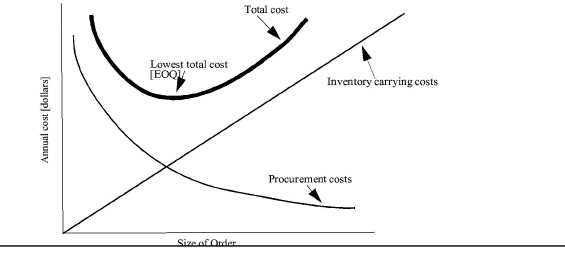
There are many different methods of determining how much inventory merchandising firms (e.g., distribu­tors, wholesalers, and retailers) should order. The best-known model used in this area is the classic eco­nomic order quantity (EOQ) model, which reveals how much to procure when a reorder point is reached. The goal of the EOQ model is to minimize the opposing costs of procuring and carrying inven­tory, as shown graphically in Exhibit 13-13

. The EOQ model assumes no stockout costs will be incurred because demand is assumed to be known and constant throughout the year.

The EOQ model is particularly applicable for independent demand items, which are free from influence of other items. For example, the demand for snow skis does not depend on the demand for refrigerators. Independent demand is fairly stable, once allowances are made for seasonal variation. Generally, indepen­dent demand items are carried on a continual basis. The EOQ in units can be calculated using the follow­ing formula:

 

where:

D = Annual demand in units

P = Cost of procuring one order

C = Annual inventory carrying costs (as a percentage of product cost)

V = Average cost or value of one unit of inventory

The EOQ formula states that the economic order quantity varies directly with demand and procurement costs and varies inversely with carrying costs. Due to the square rooting, a quadrupling of demand results only in a doubling of the EOQ.

Assume the following data: The annual demand (D) for product X is 2,400 units, and the cost of procuring (P) one order is $10. Further assume that annual carrying costs (C) are 20 percent of product cost, and the average cost or value (V) of one unit of product X is $1.50. These data are substituted in the EOQ formula as follows:

 

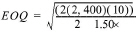
EOQ = 400 units per order, which requires six purchase orders per year to meet annual demand of 2,400 units

If the annual carrying costs per unit are known, the formula becomes:

 

where C is the annual carrying costs per unit in absolute terms. The EOQ model is based on the following assumptions:

• Only one product is involved, and it is independent of other inventory items

• A constant and known rate of demand

• A constant and known replenishment or lead time

• A stable purchase price that is independent of the order quantity or time

• A stable transportation cost that is independent of the order quantity or time

• A constant unit carrying cost

• No stockouts occur

One, however, rarely finds a situation where both demand and lead time are constant, both are known with certainty, and costs are known precisely. Fortunately, the EOQ model is relatively insensitive to small changes in the input data. Referring to the graph in Exhibit 13-13, one can see that the EOQ curve is rela­tively flat around the solution point. Although the calculated EOQ was 400 units, an EOQ variation of, say, 100 units might not change the total cost significantly. Knowing this relationship is helpful. For exam­ple, if a shipping container holds five pallets, with each pallet containing 100 units, then increasing the order to 500 units would probably be the logical decision.⁹

Adjusting the Economic Order Quantity for Volume Discounts

By ordering quantities larger than the minimum, sales quantity price discounts and transportation volume rate discounts may be available. To illustrate, refer to the EOQ calculated for product X, which was 400 units. No sales quantity price discount was available. Now assume the availability of the following sales quantity price discounts:

 

With sales quantity price discounts, the purchase price of inventory is not constant but is affected by the change in prices due to the varying discount percentages. The objective, therefore, is to identify an EOQ that minimizes not only the sum of procurement and carrying costs, but also the purchase price of inven­tory.

Exhibit 13-14

shows the effect of sales quantity price discounts. Notice that the order quantity that mini­mizes total cost (1,200 units per order) differs from the EOQ computed earlier (400 units per order) when no sales quantity price discount was available. The procurement of 400 units per order would require six orders per year. This option is not as attractive as making two orders per year at 1200 units per order. A similar analysis can be made to take advantage of transportation volume rate discounts.

Calculating the Economic Order Quantity for a Manufacturing Firm

The preceding EOQ formula is equally appropriate for calculating the optimum size of a production order or production run, sometimes called an economic batch quantity (EBQ) or economic production run (EPR). For production, V is the variable manufacturing cost per unit, and P represents an estimate of the setup cost. To illustrate, assume that stock item XYZ-8 is manufactured rather than purchased. The perti­nent input data are:

= 12,000 units

= $200 C = 30%

= $4 per unit

The optimum size of a production run is calculated as follows:

 

=

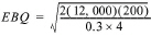
= 2,000 units per production order, which requires six production runs per year to meet annual demand of 12,000 units

Managing inventory under Uncertainty

Rarely are lead times and demand known with certainty. Consequently, management has the option of either maintaining additional inventory in the form of safety stock or incurring stockout costs. Safety stock is an amount of inventory held in excess of cycle stock (one-half of the HOQ) because of uncer­tainty in demand and lead time. This situation leads to an additional cost trade-off; that is, inventory carry­ing costs versus stockout costs. Two methods are used for managing inventory under conditions of uncertainty:

• Fixed quantity, variable period method

• Variable quantity, fixed period method¹⁰

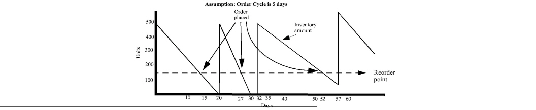
FIXED QUANTITY, VARIABLE PERIOD METHOD. Under the fixed quantity, variable period method, illustrated in Exhibit 13-15

, the order size is a fixed quantity that is placed at variable time inter­vals (the quantity may be determined by the EOQ formula). Inventory is monitored continuously, and when on-hand inventory falls to a reorder point, a fixed quantity is ordered.

The reorder point is a predetermined minimum level required to satisfy demand during the order cycle, which is five days in the example. The order cycle includes all of the time that elapses from the placement of the order until the product is received and ready for sale or usage. Order cycle is also referred to as lead time or replenishment cycle.

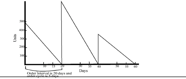
VARIABLE QUANTITY, FIXED PERIOD METHOD. Under the variable quantity, fixed period method, illustrated in Exhibit 13-16

, the order size is a variable quantity that is placed at fixed time inter­vals. Inventory is reviewed periodically, and orders are placed to bring the inventory up to some predeter­mined level.

While the two methods are mutually exclusive, it is possible to use one method with one group of inven­tory items and the other method with other groups or classes of inventory items. In general, the fixed quantity, variable period method is well suited for situations where items are ordered infrequently in large quantities compared to usage, such as with low-value items. This method works well when controlled by a computer system that monitors usage and automatically generates an order when the reorder point is reached.

The variable quantity, fixed period method is well suited for situations where groups of items are ordered for replenishment relatively frequently from one source and the inventory items are high-value items that require tight control through periodic physical checks. In this situation, more human intervention is neces­sary.¹¹

Material Requirements Planning

As described in Chapter 3, material requirements planning (MRP) is a computer-based inventory manage­ment system that focuses first on the amount and timing of finished products demanded and then computes the demand for raw materials, parts, and subassemblies at each preceding stage of production and from the vendor. Once management makes a forecast of demand for the final product, the quantities required for all components that make up that finished product can be computed based on dependent demand. All these components are dependent on the finished product. For example, an automaker's demand for four tires and a transmission depends on the production of autos. Conversely, the demand for a car is independent in the sense that a car is not a component of another product. Whereas the EOQ model focuses on inventory man­agement under conditions of independent demand, MRP focuses on inventory management under condi­tions of dependent demand.

Dependent Demand And Time-phased Procurement. The essential concepts of MRP are dependent demand and time-phased procurement (a planned amount to be ordered in each time period). Dependent demand is based on the master production schedule, which initiates and drives procurement and manufac­turing activities. Once the raw materials, parts, and subassemblies necessary to support a specific produc­tion schedule are identified, MRP provides a time-phased logic to manage their timely arrival (rather than using the reorder point described earlier in the discussion of the EOQ model).

The logic behind dependent demand is that safety stocks are not needed to support a time-phased procure­ment program such as MRP. The basic notion of time phasing is that raw materials, parts, and subassem­blies need not be carried in inventory as long as they are available when needed. Since this assumption is not always realistic, some MRP systems do allow for small safety stocks.

To gain some level of safety stocks, a common practice is to build safety time into the material require­ments plan. For example, a part may be ordered a week earlier than necessary to ensure timely arrival. Another popular approach is to increase the quantity of components by some arbitrary percentage (e.g., 5 percent) to serve as a safety stock, or cushion.

Objectives Of MRP. MRP has two primary objectives:

• Eliminate or minimize safety stocks

• Deliver raw materials, parts, and subassemblies at exactly the right time, place, and quantity needed (i.e., the JIT concept)

Because of these objectives, some companies have combined MRP with JIT.

When To Employ MRP. MRP systems are normally employed when one or more of the following condi­tions exist:

• Demand-dependent components need to be stocked only just prior to the time they will be needed in the production process.

• Large quantities of inventories are demanded at specific points in time with little or no usage at other times, such as in a job order operation as opposed to a continuous processing or mass-production opera­tion.

• All needed components can be delivered on a timely basis.

• Effective employment of the MRP system requires knowledge of the following:

• What to produce, how much, and when, as spelled out in the master production schedule

• Quantity and type of raw materials, parts, and subassemblies needed to make the finished product, as specified in the bill of materials (BOM)

• The amount of inventory in stock, as recorded in the inventory records file

• What items are on order, as listed in purchase orders outstanding

• How long it takes to get various components, as indicated by lead times compiled in the inventory records file

An MRP Example. A simplified version of a master production schedule is shown in Exhibit 13-17

. It shows planned output for finished product A. The schedule indicates that 100 units of product A will be needed for shipment to customers at the start of week 8. The master production schedule is based on what is needed, not what is possible.

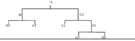
The bill of materials (BOM) contains a listing of all the raw materials, parts, and subassemblies that are needed to produce one unit of product A, as illustrated in Exhibit 13-18

. The quantity of each component that goes into the production of product A is included in parentheses. It can be readily seen that product A is composed of three B's and two C's. In addition, each B consists of three D's and two E's. Similarly, each C requires one E and two F's. Each F is made up of one G and two D's.

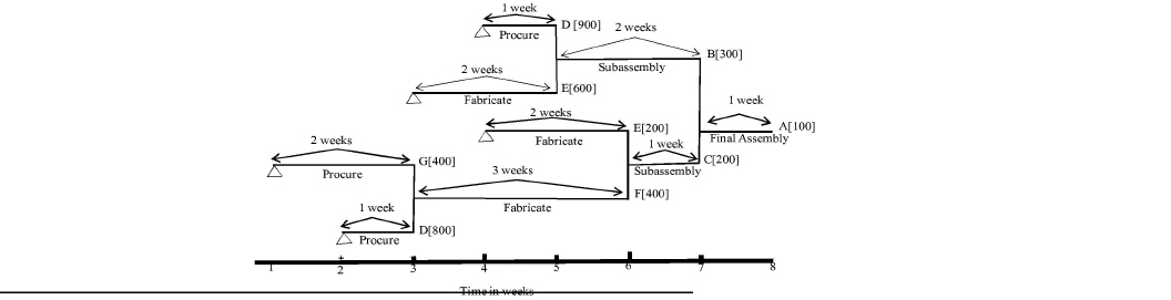
When the items are needed must be determined next. This task requires knowing the lead times, which, in turn, indicate when procuring or making the items must begin to meet the production of product A eight weeks from now. When the bill of materials is turned on its side and lead times are included, as illustrated in Exhibit 13-19

, a time-phased product structure is created.

The time-phased requirements can be readily seen in the exhibit. For example, raw material G must be ordered at the start of week 1, D at the start of week 2 and week 4. Fabrication of E and F must begin at the start of week 3, and so forth.

The quantities that were previously generated from the BOM are for gross requirements. They did not take into account any inventory that is currently on hand or due to be received. The quantities of raw materials, parts, and subassemblies that must be acquired to meet the demand generated by the master production schedule are the net requirements. Net requirements are calculated by subtracting from gross require­ments, the sum of inventory on hand and any scheduled receipts, and then adding in safety stock, if appli­cable, as shown by the following formula:

Net requirements =  Gross requirements- (On hand + Scheduled receipts + Safety stock)

In the preceding example, only item G has 100 units on hand. None of the other items are on hand or on order. The net requirements for G are:

Net requirements =  400 - (100 + 0 + 0 ) = 300 units of G

Just-in-Time

As discussed in Chapter 2, the objective of JIT, a demand-pull approach, is to reduce all inventories (raw materials, work-in-process, and finished goods) to zero or insignificant levels. JIT proponents regard inventory as a liability rather than an asset; they consider inventory a means of covering up problems. They further believe that the amount of inventory is a measure of how the organization is managed; that is, the higher the inventory amounts, the worse management's performance.

HOW JIT WORKS. If a company has eliminated its nonvalue-added activities and is practicing synchro­nized manufacturing, it can fill an order from a customer almost immediately even though there are zero inventories. The kanban at the end of the process pulls upstream activities into action, all the way back to the supplier. Because delivery from the vendor is just-in-time and the activities, such as setup, are near zero, the company becomes a high-velocity, synchronized manufacturer (a manufacturer with very short lead times) that can meet customer demands easily. High velocity is achieved by reducing setup costs, quality costs; procurement costs, and carrying costs to very low levels.

JIT AND ITS KANBAN SYSTEM. The kanban system, described in Chapter 2, is the heart of the JIT inventory management system. The kanban system PULLS the raw materials from the vendor through pro­duction and to the customer.

A kanban system uses cards that are normally inserted in a plastic envelope that is attached to a container holding the needed inventory. The kanban card is the authorization to work on or move parts. Withdrawals and replenishments occur all the way up and down the line from finished goods to vendors. The kanban system uses three cards:

• Withdrawal kanban

• Production kanban

• Vendor kanban

A withdrawal kanban specifies the quantity that a subsequent activity should withdraw from the preced­ing activity. A production kanban states the quantity that the preceding activity should produce. A ven­dor kanban specifies how many raw materials the supplier should deliver. Also stated on the vendor kanban card are the time and place of delivery.

 

A JIT EXAMPLE. Exhibit 13-20

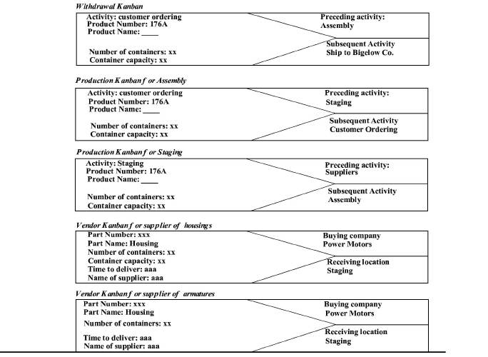
 presents examples of the three types of kanbans for Power Motors. Exhibit 13-21

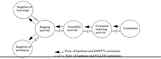
 shows the flow and linkage through-out the kanban system at Power Motors. Because JIT is a demand-pull system, the only thing that will start the production process is a customer order. The Bige­low Company sends an order for ten electric motors to the customer ordering activity of Power Motors. When the order is received, customer ordering prepares a withdrawal kanban and keeps it there for refer­ence and control. Customer ordering also prepares a production kanban and attaches it to two empty con­tainers that are transported to the assembly activity. This kanban signals the assembly activity to begin production. To do so, a production kanban must be prepared for the staging activity. This production kan­ban is attached to the two empty containers and moved to staging. Next, the staging activity prepares two vendor kanbans for delivery of ten housings and ten armatures that will be staged and assembled to make the ten electric motors ordered by Bigelow. When the parts are delivered to staging at 8:00 A.M., this first activity begins. When the first container is completed with five electric motors, the production kanban is attached to it, and it is moved to the assembly activity. When the assembly activity is completed, the con­tainer and the attached production kanban are moved to the ordering activity where the electric motors are made ready for shipment to Bigelow as soon as the second container arrives with the other five motors.

The use of kanbans ensures that a subsequent activity withdraws (or pulls) the product from the preceding activity in the required quantity at the necessary time. The kanban system, including the kanban containers and cards, controls the preceding activity by permitting it to produce only the quantities withdrawn by the subsequent activity. This way, inventories are kept at a minimum and the parts arrive just-in-time to be used.

A simple kanban system can be found in any restaurant. The customer places an order with a waiter who, in turn, gives the order to the kitchen. The meal is prepared and transferred to the waiter who checks it and gives it to the customer who ordered it. The only difference between this system and Power Motors' kan­ban system is that the waiter does not transfer a container to the kitchen. Also, suppliers for the restaurant usually deliver daily rather than at several intervals during the day.

It should be pointed out that although the goals of JIT are laudable, not all enterprises can fully implement these goals. For example, a cabinet manufacturer in Missouri cannot achieve JIT delivery from a lumber supplier located in Oregon. More than likely, the deliveries will be weekly or monthly with the size of the truckload being the most economical size to order at one time.

On the other hand, JIT is the only way some companies can operate. For example, a fish market, because of the perishability of its product, must operate according to JIT principles.

Measuring Inventory Management Effectiveness and Efficiency

No matter which inventory management approach is used (i.e., EOQ, reorder point, and safety stock; MRP; or JIT), almost every enterprise, at one time or another, is faced with the problems of surplus, short, incorrect, and obsolete inventory and inadequate attention to high-value items. Whatever the reasons for such conditions, the management accountant must provide information that will help management take corrective action to manage inventory more effectively and efficiently. Two methods can be used to pro­vide such information:

• Contribution-by-value analysis

• Turnover ratios

USING THE CONTRIBUTION-BY-VALUE ANALYSIS METHOD. One of the simplest and most effective ways to manage inventories efficiently is the contribution-by-value analysis method (also called the ABC analysis method), which is based on Pareto's principle, as presented in Chapter 12. This law states that in most situations a relatively small percentage of certain objects contributes a relatively high percentage of output.

For example, review the contribution-by-value analysis report in Exhibit 13-22

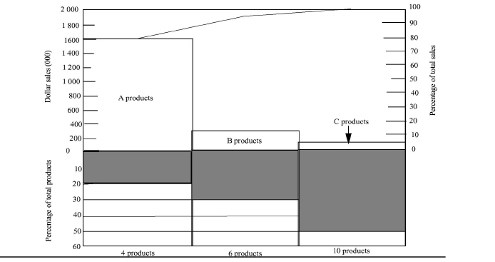
. This report reveals that A items account for 20 percent of the products in inventory but contribute 80 percent of sales. The B items account for 30 percent of the products and add an additional 15 percent of sales. The C items account for 50 percent of the products but add only 5 percent of sales. The Pareto chart in Exhibit 13-23

 presents a visual interpretation of the information in the contribution-by-value analysis report.

For the A items, management should provide sufficient safety stocks and high levels of service. B items should receive less attention and probably lower or zero safety stocks. As for the C items, management may actually consider eliminating some of the products from inventory because their contribution to sales revenue is minimal.

USING TURNOVER RATIOS. Ratios are one of the most common methods for measuring inventory management effectiveness and efficiency. The following are typical turnover ratios:

Raw materials = Cost of raw materials used  / Average raw materials inventory

Work-in-process = Cost of goods manufactured / Average work-in-process inventory

Finished goods = Cost of goods sold / Average finished goods inventory

The data for these turnover ratios are derived from financial accounting data. Thus, they are influenced by the financial accounting procedures used for measuring periodic income. For example, a writedown of inventory will usually be charged against cost of goods sold so that the writedown, which may be an indi­cator of inventory inefficiency, will actually increase inventory turnover. Also, the various inventory cost­ing procedures (e.g., FIFO, LIFO) make interpretation of inventory turnovers very complex. For example, how does one interpret the turnover ratio of the current cost of goods sold to the average inventory costed by the LIFO inventory costing procedure when LIFO inventory may be costed at prices that occurred many years ago? Moreover, there is a problem of aggregating data. For instance, a moderately rapid turnover ratio for the inventory may obscure the fact that half of the inventory is turning very slowly and the other half very rapidly.¹²

Calculating turnover ratios on a unit basis helps minimize the preceding problems and makes the ratios more meaningful. For an individual product, the inventory turnover is the ratio of the number of units sold or issued to the average number of units on hand, such as:

Product X Turnover Ratio =

= # of units of product X sold during the month / Average # of units of product X on hand during the month

Assume 1,200 units of product X were sold during March. At the beginning of March, 500 units were on hand, and at the end of March, 300 units were on hand, giving an average number of units on hand during March of 400 [(500 + 300) = 2]. Thus, the turnover ratio of product X is 3, calculated as follows:

Product X Turnover Ratio = 1,200 units of product X / 400 average units on hand

= 3 turns during March

Turnover ratios should be used only as indicators. Using them as a sole measure of inventory management effectiveness and efficiency can backfire. For example, the traditional assumption is that the higher the turnover, the better. A better goal may be to carry zero inventory. In a JIT environment, this is the goal. In other environments that depend on some amount of inventory on hand, a zero-inventory policy would cause problems, such as stockouts and excessive procurement costs. Any meaningful application of turn­over ratios must, therefore, implicitly assume that high turnovers are only desirable to the extent that they are compatible with effective and efficient operations. Inventory turnovers are worth improving only if there is no substantial increase in procurement costs or significant loss of sales resulting from excessive stockouts. Turnover ratios are only useful if they can be related in some way to inventory management costs and the optimum decisions of how much and when to order.¹³

MANAGING WAREHOUSING COSTS

LEARNING OBJECTIVE 5

Warehousing is the link between the producer and the customer. It is the activity in the logistics system that stores products (raw materials, parts, supplies, subassemblies, work-in-process, finished goods) at and between the point-of-origin and point-of-consumption.

What Are the Reasons for Warehousing?

In general, the warehousing of inventories is necessary for the following reasons:

• To achieve transportation economies

• To achieve production economics

• To maintain a source of supply

• To meet changing market conditions (e.g., seasonality and demand fluctuations)

• To achieve a desired level of customer service¹⁴

Costing and Budgeting Warehousing Activities

Warehousing is a major activity in many logistics systems. The warehousing activity itself consists of spe­cific activities, such as receiving; storing; order picking, packing, and staging; and shipping.

A management accounting system should produce a variety of performance measurements to help manag­ers examine warehousing productivity. For instance, financial performance measurements include the fol­lowing:

Receiving and storage cost per unit =

   = Total receiving and storage costs per week / Avg # of units stored per week

   = $2,400 receiving and storage costs / 8,000 units stored

   = 0.30 $/unit

Picking costs per unit =

   = Total picking costs per week / Number of units picked per week

   = $1,200 picking costs / 6,000 units picked

   = 0.20 $/unit

Packing costs per unit

   = Total packing costs per week / Number of units packed per week

   = $6,000 packing costs / 6,000 units packed

   = 1.00 $/unit

Staging costs per shipment

   = Total staging costs per week / Number of shipments staged per week

   = $80,000 staging costs / 4,000 shipments staged

   = 20.00 $/shipment

Loading costs per shipment =

   = Total loading costs per week / Number of loads per week

   = $200,000 loading costs / 2,000 loads

   = 100 $/load

Demurrage costs (i.e., the costs for detaining a transportation vehicle) are also important. Increasing demurrage costs indicate poor dock scheduling for inbound and outbound shipments. Performance mea­surements for inbound and outbound shipments can be calculated in the following manner:

Inbound demurrage costs per load =

   = Total inbound demurrage costs per week / # of loads rec’d in the week

   = $20,000 inbound demurrage costs / 100 inbound loads

   = 200 $/inbound load

Outbound demurrage costs per load =

   = Total outbound demurrage costs per week / # of loads shipped in the week

   = $30,000 outbound demurrage costs / 200 outbound loads

   = 150 $/outbound load

Can the Procurement and Warehouse Activities Be Eliminated?

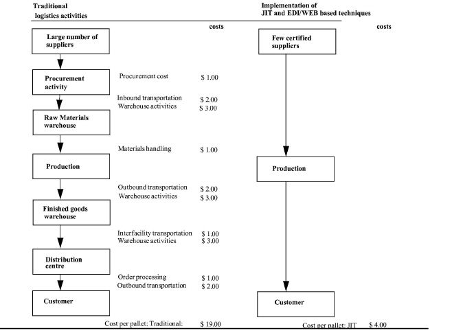
Clearly, procurement and warehouse activities add costs incrementally to products. By applying JIT and EDI techniques, these activities can be reduced or eliminated, as illustrated in Exhibit 13-24.

By using JIT and EDI techniques, the procurement activity can be eliminated, along with the $1.00 per pallet cost. Direct delivery of raw materials to production eliminates the warehouse activities cost of $3.00 per pallet and the materials handling cost of $1.00 per pallet. Similarly, transportation to the finished goods warehouse, finished goods warehouse activities, interfacility transportation, distribution center warehouse activities, and order processing activities, which incur a combined cost of $10.00 per pallet, can be eliminated with JIT and EDI. In fact, JIT and EDI techniques help reduce overall costs by $15.00 per pallet ($19.00 - $4.00).

Not all companies can take full advantage of JIT and EDI techniques, however, especially those that expe­rience marked seasonality in production or sales patterns. In fact, some companies such as food processors must stockpile raw materials and run production full-time during a two- or three-month period immedi­ately after the crop is harvested. After the products are packed, food processing companies must store the products in warehouses throughout the year until they are sold.

Similarly, the seasonal requirements for toys and clothing usually cannot he supplied by current production capacity. Therefore, many companies use warehousing to store products in advance of heavy selling sea­sons in order to facilitate smooth production throughout the year.

SUMMARY OF LEARNING OBJECTIVES

The major goals of this chapter were to enable you to achieve five learning objectives:

Learning objective 1. Discuss how an electronic data interchange (EDI) system can support logistics and reduce costs.

An EDI system embedded in the integrated computer-based information system (ICBIS) acts as a nerve center for the logistics system. Information from the ICBIS helps to coordinate all the logistics activities. Implementing EDI into the ICBIS provides the potential to increase logistics productivity and thereby reduce total costs.

A high-quality, last information flow facilitates the integration of all logistics activities. Conversely, a poor flow of information, which can allow lost orders, bottlenecks, and errors to go undetected, can create confusion and inefficiencies within the logistics system.

The cost associated with achieving a rapid flow of error-free information is more than offset by cost sav­ings realized throughout the logistics system. For example, assume that servicing a customer requires four days for order transmittal and processing, two days for warehouse processing, and one day for air freight transportation. An investment in an EDT system could reduce transmittal and processing time to one day. With the five extra days gained from this efficiency, the company can choose a less expensive transporta­tion mode or improve customer service, thus differentiating itself from its competitors.

Learning objective 2. Define procurement, and explain how procurement costs can be reduced.

Procurement costs are incurred to get the right product to the right place at the right price and at the right time. Because procurement costs represent a substantial cost of doing business, this activity's performance should be measured. Implementing JIT techniques can help reduce procurement costs. Traditionally, the buying company has assumed the role of monitoring the quality of purchased materials, inspecting and counting materials for quality and quantity, and returning poor-quality materials to the supplier for rework and adjustments. The ultimate goal of the buying company is to be able to certify suppliers as sources of high-quality materials and thus eliminate all the preceding nonvalue-added activities associated with pro­curement.

Learning objective 3. Describe the transportation activity, and examine how pro­ductivity of this activity can be increased.

Transportation, together with warehousing, adds time and place utility to products. The five basic modes of transportation-motor, rail, air, water, and pipeline-provide movement of products between where they are produced and where they are consumed. Each mode has different cost and service characteristics.

Typically, transportation costs are assigned to loads, shipments, and products for costing purposes. Also, a variety of performance reports and measurements help management increase transportation productivity.

Learning objective 4. Explain how to manage inventory costs.

The objective of managing inventory costs is to maintain the lowest possible inventory consistent with customer service and production goals. This objective revolves around two decisions:

• How much to order or produce

• When to order or produce

Three inventory management approaches help deal with these decisions:

• EOQ, reorder point, and safety stock

• MRP

• JIT

Inventory costs include:

• Procurement (or setup) costs

• Carrying costs

• Stockout costs

The EOQ model minimizes the total of carrying costs and procurement (or setup) costs. Managing inven­tory under uncertainty entails minimizing the trade-off between carrying costs and stockout costs. Two methods are used to do this:

• Fixed quantity, variable period method

• Variable quantity, fixed period method

The MRP and JIT approaches to inventory management seek to overcome assumptions regarding stable usage and independent demand that are required for EOQ calculations. Whereas EOQ calculations result in a uniform order quantity that may be ordered in a fixed or variable time interval, the order sizes gener­ated by MRP and JIT are more flexible to accommodate irregular usage.

MRP and JIT approaches are used primarily by manufacturers that make products that are dependent on other components. For example, the production of a leaf blower requires a motor and various parts that must be procured or made. All of this inventory that is, the leaf blower (the finished product) and its vari­ous components (raw materials, parts, and subassemblies)—is not made or ordered until needed. Thus, the MRP and JIT approaches are based on demand-pull and just-in-time concepts that minimize or eliminate all inventories.

For MRP and JIT to work, all activities of the logistics system must be fully integrated and efficient. A weak link in the logistics chain can spell disaster for either inventory management approach. For example, transportation becomes an even more critical activity under MRP and JIT. Although warehousing is reduced under MRP and JIT, a relatively small facility may be needed to consolidate and stage raw materi­als for input to production and output finished goods for shipping to external customers.

Two key methods are used to measure inventory management effectiveness and efficiency:

• Contribution-by-value analysis method

• Turnover ratios

Learning objective 5. Describe the warehousing activity, and explore ways to man­age warehouse costs.

The purpose of warehousing is to provide place and time utility for inventory management. The relative importance of warehousing, however, varies among companies.

A number of performance measurements should be prepared to help manage specific warehousing activi­ties effectively and efficiently. In companies where JIT and EDI techniques are implemented, procurement and warehousing activities can be reduced, if not eliminated, thus reducing a substantial amount of logis­tics costs while increasing the effectiveness and efficiency of the logistics system.

IMPORTANT TERMS

Contribution-by-value analysis method (ABC analysis method) A method based on Pareto's principle, which states that a relatively small percentage of certain objects contributes a relatively high per­centage of output.

Cycle stock An amount of inventory equal to half the economic order quantity.

Dependent demand A situation where the demand for raw materials, parts, and subassemblies is derived from plans to make certain finished products.

Economic order quantity (EOQ) model A formula for minimizing inventory carrying and procurement costs. The EOQ model can also be used to calculate the optimum size of a production order.

independent demand A situation where inventory items are not connected or related to each other.

Inventory carrying costs Expenditures incurred for holding inventory.

Logistics costs Expenditures incurred for planning, implementing, controlling, and operating all logistics activities.

Logistics systems Represent the integration of procurement, transportation, inventory management, and warehouse activities to provide the most cost-effective means of meeting internal and external customer requirements.

Order cycle (lead time or replenishment cycle) Includes all the elapsed time from placement of an order until the product is received and ready for sale or usage.

Procurement A logistics activity that includes purchasing and receiving verification of inbound raw mate­rials or products.

Procurement costs Expenditures incurred either for placing purchase orders with suppliers and receiving inventory or for preparing work orders for ordering a production lot and setting up for production.

Production kanban States the quantity that the preceding activity should produce.

Reorder point A predetermined minimum level required to satisfy demand during the order cycle.

Safety Stock An amount held to protect against demand and order cycle (lead time) variabilities.

Stockout costs Expenditures incurred for not having inventory available when needed.

Time-phased procurement A planned amount of raw materials, parts, and subassemblies to be ordered or fabricated in each time period.

Transportation A logistics activity that involves movement of materials and products from origin to desti­nation.

Vendor kanban Specifies how many raw materials the supplier should deliver.

Warehousing Serves as a link between the producer and the customer. Specific activities include receiv­ing; storage; order picking, packing, marking, and staging; and shipping.

Withdrawal kanban Specifies the quantity that a subsequent activity should with-draw from the preced­ing activity.

DEMONSTRATION PROBLEMS

DEMONSTRATION PROBLEM I Preparing driver productivity and fuel reports.

Matthews arid Butch Smith are truck drivers for Cleveland Express. Data related to their performance during June 19X4 follow:

 

Required:

a. Prepare a driver productivity report for the month. The total standard miles that a driver is supposed to operate per month is 9,500 miles. The standard load ratio is 80%.

b. Prepare a driver fuel report for the month. The standard miles per gallon (MPG) is 4.9; the standard cost per gallon is $1.30.

SOLUTION TO DEMONSTRATION PROBLEM 1 a.

 

b.

DEMONSTRATION PROBLEM 2 Determining the EOQ and order cycle for a distributor.

Big-O, a local distributor for a national tire company, expects to sell approximately 10,000 low-ride tires of a certain size next year. Annual carrying costs are $10 per tire, and procurement costs are $80 per order. The distributor operates 300 days a year.

Required:

a. Determine the EOQ.

b. How many times a year should the store reorder?

c. Determine the length of an order cycle.

SOLUTION TO DEMONSTRATION PROBLEM 2

a.  =  =

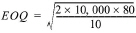= 400 tires

b. Number of orders per year:

D/ EOQ = 10,000 tires / 400 tires = 25 orders per year

c. Length of order cycle:

EOQ / D = 400 tires / 10,000 tires = 4% of the distributor's year

or,

4% x 300 days = 12-day order cycle (or lead time)

Thus, on the average, it must take 12 workdays from the placement of the order until the tires are received and ready for sale with an EOQ of 400 tires and a demand of 10,000 tires.

DEMONSTRATION PROBLEM 3 Calculating an EOQ in which carrying costs are stated as a percent­age of the purchase price of an item rather than as a dollar amount per unit.

The Master's Voice TV Company plans to purchase 5,000 picture tubes a year at $150 each. Procurement costs are $30, and annual carrying costs are 20% of the purchase price.

Required:

a. Calculate the EOQ.

b. Calculate the total annual cost of procuring and carrying the picture tubes.

SOLUTION TO DEMONSTRATION PROBLEM 3.

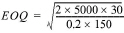 = = 100 picture tubes

b. Total annual costs = Procurement costs + Carrying costs

= (D/EOQ) x P + (EOQ/2) x CV

= (5,000/100) x $30 + (100/2) x .20($150) = $1,500 + $1,500 = $3,000

Notice that the procurement and carrying costs are equal at the EOQ, which is at the optimum point (or minimum total cost point).

DEMONSTRATION PROBLEM 4 Calculating the reorder point.

The invoice printing operation at Sierra Power Company uses three boxes of printer paper per day. 1t takes the supplier five days to deliver an order of printer paper.

 

Required:

Determine at what point Sierra should place its order.

SOLUTION TO DEMONSTRATION PROBLEM 4

Usage = 3 boxes per day

Lead time = 5 days

Reorder point = Usage x Lead time

= 3 boxes per day x 5 days = 15 boxes

Therefore, Sierra should recorder when 15 boxes are left in inventory.

DEMONSTRATION PROBLEM 5 Calculating an EOQ (or EBQ) for a manufacturer.

Storite makes plastic filing cabinets for floppy disks. The management accountant has collected the fol­lowing data:

• Setup cost $500 per batch

• Carrying cost $20 per unit per year

• Expected annual demand 5,000 units

Required:

Compute the EOQ (or EBQ) and explain what it means.

SOLUTION TO DEMONSTRATION PROBLEM 5

EOQ = 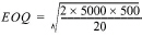= 500 units per batch

The optimal decision is to produce 500 units at a time, which means that there will be 10 production runs (or batches) per year (5,000 units annual demand / 500 units produced per run). The EOQ means that car­rying costs equal setup costs as indicated below:

Carrying costs = (500/2) x $20    = $ 5,000

Setup costs = (5,000/500) x $500   = $ 5,000

Total costs    = $10,000

DEMONSTRATION PROBLEM 6 Calculating the EOQ, safety stock, and lead time.

Humdinger Trucks purchases motors from Birmingham Diesel. The plant manager is trying to determine the lot size that should be ordered so as to minimize the sum of carrying and setup costs. She also wants to avoid stockouts, since any stockout would shut down the assembly line. To help her make her decision, you have supplied the following data:

• Annual demand for motors: 20,000

• Unit carrying cost: $100

• Setup cost: $900

• Average demand for motors: 65 per day

• Maximum demand for motors: 70 per day

• Lead time: 5 days

Required:

Calculate the EOQ, safety stock, and reorder point for the plant manager.

SOLUTION TO DEMONSTRATION PROBLEM 6

 

EOQ = 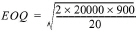 = 600 motors per run

Safety stock:

Reorder point = (Average usage x Lead time) + Safety stock =

= (65 x 5) + 25 = 350 motors remaining in inventory

DEMONSTRATION PROBLEM 7 Making an ABC analysis. The following data represent annual sales at the Chic Boutique

 

Required:  

Using a bar graph, classify the inventory items as A, B, or C based on annual dollar sales value.

SOLUTION TO DEMONSTRATION PROBLEM 7

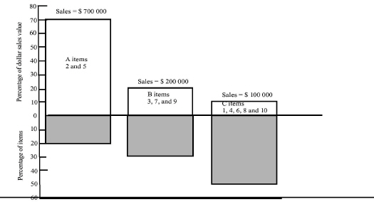
REVIEW QUESTIONS

13.1 The management of inventory costs revolves around two decision criteria. Name them.

13.2 Ignoring safety stock, which of the following is a valid computation of the reorder point?

a. The economic order quantity.

b. The economic order quantity multiplied by the anticipated demand during the lead time.

c. The anticipated demand during the lead time.

d. The square root of the anticipated demand during the lead time.

13.3 What is the difference between the EOQ model for merchandising firms and the EOQ model for man­ufacturing firms?

13.4 What are the main reasons that an organization has inventory?

13.5 What are the assumptions of the EOQ model?

13.6 A decrease in carrying costs will:

a. Increase the safety stock required.

b. Decrease the economic order quantity.

c. Have no effect on the economic order quantity.

d. Increase the economic order quantity.

e. Decrease the number of orders issued per year.

13.7 Safety stocks are used to compensate for:

a. Variability in inventory demand rates and lead time.

b. Variability in inventory prices and lead tithes.

c. Variability in inventory demand rates and prices.

d. Inventory obsolescence and sales returns.

e. Variability in customer needs and inventory pricing.

13.8 A company would use the EOQ model to:

a. Minimize the unit purchase price of inventory.

b. Minimize the number of orders placed during the year.

c. Minimize the cost of placing orders.

d. Minimize the combined costs of placing orders and carrying inventory.

e. Minimize the required amount of safety stock.

13.9 The inventory management model that follows Pareto's principle is the:

a. Economic order quantity (EOQ) model.

b. Material requirements planning (MRP) model.

c. ABC analysis model.

d. Just-in-time (JIT) model.

e. Lead time model.

13.10 When the level of safety stock is increased:

a. Lead time will increase.

b. Lead time will decrease.

c. The frequency of stockouts will decrease.

d. Carrying costs will decrease.

e. Procurement costs will decrease.

13.11 Describe how EDI enhances the logistics system.

13.12 Discuss the types of information bar codes provide in an EDI system. 13.13 Identify four goals of the procurement function.

13.14 Name two characteristics of JIT procurement in relation to supply, quantity, and quality consider­ations.

13.15 Which of the following is not a benefit of AT procurement to the supplier?

a. Reduced nonvalue-added activities.

b. Increased ability to predict resource arid capacity needs.

c. Increased inventories.

d. Reduced labor force.

e. Increased control over outbound shipments.

13.16 What arc the three cost drivers of transportation costs?

13.17 Name the three cost objects to which transportation costs are normally assigned.

13.18 Name the three popular approaches to inventory management.

13.19 The simple economic production run model will only apply to situations in which the production rate:

a. Equals the demand rate,

b. Is less than the demand rate.

c. Is greater than the demand rate.

d. Exceeds the supply rate.

e. For the period covered equals the projected sales for the period.

13.20 Which one of the following items is not included in the annual carrying costs of inventory?

a. Cost of capital.

b. Insurance on inventory.

c. Annual warehouse depreciation.

d. Taxes on inventory.

e. Inventory breakage on stored inventory.

13.21 Contrast independent and dependent demand. Give an example of each.

13.22 When is it appropriate to employ MRP?

13.23 Which one of the following is not a benefit of JIT inventory management?

a. Increased cash discounts on purchases.

b. A reduction in the number of suppliers.

c. A reduction in procurement costs.

d. Less checking on quality and quantity of delivered raw materials.

e. A reduction in the total value of inventories on hand.

13.24 If one optimizes the inventory turnover ratio for a particular item, which costs will not increase?

a. Total reorder costs.

b. Stockout costs.

c. Unit reorder costs.

d. Carrying costs.

e. Procurement costs.

13.25 Which condition would justify accepting a low inventory turnover ratio from the viewpoint of inven­tory management?

a. High obsolescence costs.

b. High carrying costs.

c. High stockout costs.

d. Short lead times.

e. Low procurement costs.

13.26 Name four types of stockout costs.

13.27 What are the two primary objectives of MRP?

13.28 What condition(s) should exist before MRP is used?

13.29 The kanban system uses three cards. Name them and describe the information they contain.

13.30 What is the primary benefit of using a kanban system?

13.31 What are the main reasons that an organization uses warehousing?

CHAPTER-SPECIFIC PROBLEMS

These problems require responses based directly on concepts and techniques presented in the text.

13.32 Calculating performance measures to help manage procurement costs. Magna Distributors pro­cessed 8,000 purchase orders last year using ten purchasing agents. This year Magna processed 10,000 purchase orders employing eight purchasing agents. Administrative costs were $480,000 last year; this year, they are $460,000. Last year, 900 production orders were released, and there were 18 complaints associated with these orders. This year, 1,200 production orders were released, and there were 48 com­plaints associated with these orders.

Required: Calculate performance measures for the preceding situation, and discuss what the results may be indicating to management.

13.33 Determining characteristics of JIT procurement. Following is a random list of characteristics that may or may not be applicable to JIT procurement:

• Large number of suppliers.

• Short-term contracts. Certified suppliers.

• Suppliers scattered throughout the country.

• Frequent deliveries in small quantities.

• High quality of incoming materials.

• Excessive amount of record keeping.

• Close relationship with suppliers.

• Price is the primary criterion used to select suppliers.

Required: Identify each with a T for true or an F for false.

13.34 Determining certified supplier benefits of JIT procurement. Following is a random list of items that may or may not be applicable to a certified JIT supplier:

• More paperwork.

• Reduced long-term risk of doing business.

• Reduced ability to predict resource and capacity needs.

• Does not participate with buying company's new product development team.

• Less supervision.

• Increased control of finished goods.

• Reduced work-in-process and finished goods carrying costs.

• More labor.

• Increased ability to plan ahead for design changes.

• Increased ability to retain a trained labor force.

Required: Identify each with a T for true or an F for false.

13.35 Assigning load costs to shipments. The Top Speed Trucking Company's management accountant is conducting an analysis of the company's transportation costs. He has collected the following data for one day:

 

Total load costs = $8,700

Required:

a. Calculate the cwt-miles per shipment.

b. Calculate the percentage of total cwt-miles.

c. Assign the shipment costs.

(Note: Do not consider “empty backhaul miles.”)

13.36 Calculating performance measurements for the transportation activity. The Tranzsport-It-All Company has gathered the following information, which it plans to use in evaluating the efficiency and effectiveness of its transportation activity over the past fiscal year:

Number of shipments 667,000; Total miles shipped 500,000; Total tons shipped 470; Number of customer complaints 51,000; Number of damage claims 28,000; Number of late deliveries 121,000; Total transpor­tation costs $8,000,000

Required: Calculate the following performance measurements for the procurement activity:

a. Customer complaints.

b. Damage claims.

c. Late deliveries.

d. Cost per ton-mile.

13.37 Classifying inventory costs. Following are a variety of costs:

• Purchase order forms.

• Telephone call to a vendor.

• Purchasing agent's salary.

• Wages of receiving personnel.

• Parts awaiting use.

• Profit lost due to inventory nonavailability.

• Preparing and issuing checks to suppliers.

• Production setups.

• Money invested in inventory.

• Ad valorem taxes.

• Insurance premiums for inventory on hand.

• Security measures.

• Freight for relocating inventory.

• Postage for purchase orders.

• Property taxes on warehouses.

• Disposal of inventory at a price less than its cost.

• Wages for inventory record keeping.

• Shipping charges for rush orders.

• Losses due to theft.

• Costs of handling backorders.

Required: Indicate whether each of the preceding costs would be considered a cost of ordering (O); that is, a procurement or setup cost; a cost of carrying (C); or a cost of stockout (S).

13.38 Calculating the reorder point. The Cartex Company uses a part to which the following data are applicable:

 

Units of the part will be required evenly throughout the year.

Required: Calculate the reorder point.

13.39 Determining the reorder point. Ritenice Pen Company uses an average of 400 ink inserts per day, and lead time averages five days. Because both usage rate and lead times are variable, Ritenice carries a safety stock of 500 ink inserts to reduce the chance of a stockout.

Required: Determine the reorder point.

13.40 Calculating the EOQ. The Family Clothing Store sells three main products: pants, dresses, and shoes. The following data are available on each product:

 

Required: Calculate the EOQ for each product.

13.41 Determining annual carrying cost per unit. [CMA adapted] Hector Motors, Inc., is a single-product company. Various annual costs relating to its product follow:

• Cost per unit:

• Freight-in on purchases $0.20

• Storage 0.12

• Insurance 0.10

Total per year:

Interest that could have been earned on alternate investment funds   $800

Units required   10,000

Required: Determine the annual carrying cost per unit.

13.42 Analyzing an EOQ diagram. [CMA adapted] The accompanying diagram represents the EOQ model:

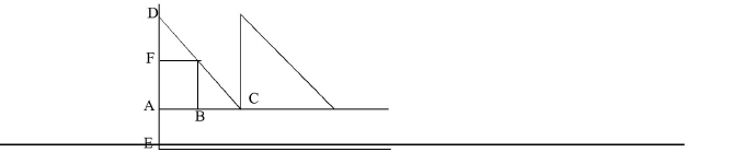
Required:

a. Which line segment represents the reorder lead time?

b. Which line segment identifies the quantity of safety stock maintained?

c. Which line segment represents the length of time to consume the total quantity of materials ordered?

13.43 Determining material requirements in an MRP system. Following is a bill of materials (BOM) for product A:

 

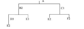
Required:

a. Determine the gross material requirements for B, C, D, E, and F to make one unit of product A.

b. Determine the gross material requirements to produce 100 units of product A.

c. Assume that D has 100 on hand and E has 300 on hand, 200 scheduled to be received (i.e., on order), and 100 in safety stock. Calculate the net material requirements for D and E. None of the other compo­nents have any inventory on hand, on order, or in safety stock.

13.44 Cost savings resulting from increasing the turnover rate. [CMA adapted] Markquic Company's budgeted sales and budgeted cost of sales for the coming year are $144,000,000 and $90,000,000, respec­tively. Short-term interest rates are expected to average 10%.

Required: If Markquic can increase inventory turnover from its present level of 9 times per year to a level of 12 times per year, what cost savings would be expected in the coming year?

13.45 Identifying concepts associated with MRP. Following are various concepts that may or may not be associated with MRP:

• Lead time

• Inventory levels

• Bill of lading

• Dependent demand

• Bill of materials

• Independent demand

Required:

Insert a T for true for each concept that is associated with MRP and an F for false for each concept that is not.

13.46 calculating turnover ratios. The management accountant at Z-Bender Company has gathered the following data on Z-Bender's inventories to assist him in evaluating the effectiveness and efficiency with which its inventories are being managed:

Number of units sold of product Z 14,700; Cost of goods sold $70,300; Cost of goods manufactured $44,000; Cost of raw materials used $27,500; Average number of units on hand of product Z 4,900; Aver­age finished goods inventory $21,300; Average work-in-process inventory $11,000; Average raw materi­als inventory $6,000.

Required:

Calculate the turnover ratios for:

a. Raw materials.

b. Work-in-process.

c. Finished goods.

d. Product Z.

13.47 Calculating financial performance measurements to determine warehousing productivity. The management accounting system at Triostep Company has accumulated the following warehousing-related information in its database for the prior month:

 

Required: Calculate the following financial performance measurements:

a. Receiving and storage costs per unit.

b. Picking costs per unit.

c. Packing costs per unit.

d. Staging costs per shipment.

e. Loading costs per shipment.

f. Outbound demurrage costs per load.

THINK-TANK PROBLEMS

Although these problems are based on chapter material, reading extra material, reviewing previous chap­ters, and using creativity may be required to develop workable solutions.

13.48 Determining the impact of transportation volume rate discount. O'Leary Wholesalers has collected the following data on its product A:

Required:

a. Calculate the EOQ using the above data.

b. Assume that the most desirable transportation rate is achieved when a quantity of 900 units is ordered as compared to the EOQ-recommended order calculated in Requirement (a). Also assume that the transporta­tion rate for the EOQ is $1.80 per unit, but if the order is 900, the rate drops to $1.45 per unit. Explain the impact of this transportation volume rate discount. Taking into consideration the potential transportation savings by purchasing in 900-unit lot sizes, determine the cheapest way to order product A.

13.49 Calculating expected usage. [CMA adapted]  Compurite Computer Company began producing lap­top computers last year. At that time the company forecasted the need for 10,000 integrated circuits annu­ally. During the first year, the company placed orders when the inventory dropped to 600 units so that it would have enough to produce laptops continuously during a three-week lead time. Unfortunately, the company ran out of this component on several occasions, and costly production delays resulted. Careful study of last year's experience resulted in the following expectations for the coming year:

 

The study also suggested that the usage during a given week was statistically independent of usage during any other week and usage was also statistically independent of lead time.

Required:

a. Calculate the expected usage during a regular production week.

b. Calculate the expected usage during lead time,

c. If the company reorders integrated circuits when the inventory has dropped to a level of 700 units, what is the probability that it will run out of this component before the order is received?

13.50 Determining Procurement And Carrying Costs. [CMA adapted] Toyland is a wholesale distributor of toys. The company leases space in a public warehouse and is charged according to square feet occu­pied. Toyland has decided to employ the EOQ formula to determine the optimum number of cases of toys to order.

The company placed 2,400 orders last year. Data for the high-activity month, low-activity month, and the year for the procurement and warehouse operations are as follows:

 

The annual charges for the warehouse totaled $12,750 last year. In addition, the annual insurance and property taxes on the toys stored in the warehouse amounted to $1,500 and $2,250, respectively. The aver­age monthly inventory last year was $75,000.

Long-term capital investments are expected to earn 12% after income taxes. Toyland is subject to an effec­tive income tax of 40%.

Required:

a. Determine the variable cost of placing an order that would be used in the EOQ formula.

b. Determine the annual carrying cost, stated as a percentage, that would he used in the EOQ formula.

13.51 Computing EOQ and safety stock. [CMA adapted] Clyde Peterson, general manager for Adam Desk Company, is exasperated because the company exhausted its finished goods inventory of Style 103-Modern Desk twice during the previous month. This led to customer complaints and disrupted the normal flow of operations.

“We ought to be able to plan better,” declared Peterson. “Our annual sales demand is 18,000 units for this model or an average of 75 desks per day based upon our 240-day work year. Unfortunately, the sales pat­tern is not this uniform. Our daily demand on that model varies considerably. If we do not have the units on hand when a customer places an order, 35% of the time we lose the sale, 40% of the time we pay an extra charge of $24 per unit to expedite shipping when the unit becomes available, and 25% of the time the customer will accept a backorder at no out-of-pocket cost to us.

“When we run out of units, we cannot convert immediately because we would disrupt the production of our other products and cause cost increases. The setup process for this model results in the destruction of 12 finished desks, leaving no salvageable materials. Once we get the line up, we can produce 200 units per day. I would prefer to have several planned runs of a uniform quantity rather than the short unplanned runs often required to meet unfilled customer orders.”

The management accountant has suggested that the company adopt an EOQ model to determine optimum production runs and then establish a safety stock to guard against stockouts. The cost data for the Modern Desk, which sells for $110, are readily available from the management accounting records. The manufac­turing costs are as follows:

The management accountant estimates that the company's carrying costs are 19.2% of the incremental out-of-pocket manufacturing costs. This percentage can be broken down into a 10.8% variable rate and an 8.4% fixed rate.

The EOQ formula referred to by the management accountant is as follows:

 

where

D = Annual demand in units

C = Cost of placing an order

K = Annual unit cost of carrying inventory

Required:

a. Adam Desk Company can solve part of its production scheduling problems by adapting the EOQ model to determine the optimum production run.

1. Explain what costs the company would be attempting to balance when it adapts the EOQ model to pro­duction runs.

2. Calculate the optimum quantity that Adam Desk Company should manufacture in each production run of Style 103-Modern Desk.

3. Calculate the number of production runs of Modern Desks that Adam Desk Company would schedule during the year based upon the optimum quantity calculated in Requirement (a)2.

b. Adam Desk Company should establish a safety stock level to guard against stockouts.

1. Explain what factors affect the designated size of the safety stock for any inventory item.

2. Calculate the minimum safety stock level that Adam Desk Company could afford to maintain for the Style 103-Modern Desk and not be worse off than if it were unable to fill orders equal to an aver­age day's demand.

13.52 Discussing the implementation of JIT. [CMA adapted] Over the past several years, many compa­nies have decided to implement a JIT production system. They have met with varying degrees of success because implementation of J1T is dependent on many factors such as management commitment to and employee acceptance of the process. In addition, a company must be willing to change the way it thinks about its employees, suppliers, and customers if it is going to be successful in using JIT procedures.

Required:

a. In general, describe several actions that a company can take to facilitate an organizational change.

b. To ensure the success of a JIT production system, describe the relationship a company must establish with its:

1. Suppliers.

2. Customers.

3. Employees.

c. The success of a JIT production system requires changes in management skills and behavior.

1. Describe at least two changes in management skills and behavior that will be required to ensure a successful transition to a JIT production system.

2. Identify several steps a company can take to achieve the changes described in Requirement (c) 1.

13.53 Analyzing Procurement Costs. The Premier Cuisine Restaurant Company owns and operates seven different restaurants in the San Francisco Bay area. The purchasing function is centralized in the down­town San Francisco home office. The company also has one centralized warehouse. The warehouse man­ager recently voiced concern to management regarding the broad types of glassware being carried in inventory, many of which contained specialized logos and many of which are no longer being used in the restaurants. He also expressed concern that he continues to receive orders for specialized glassware from each restaurant, thus, further building up the diverse glassware inventory as well as keeping unit costs high. Management asked that the warehouse manager provide them with a breakdown of the number of different types of glassware currently in stock by major glassware type. The following data were provided to management:

 

When management reviewed these data with purchasing, it was also found that this glassware had been ordered from a total of 13 vendors.

Required:

a. Identify the primary weaknesses or diseconomies with the company's current procurement function.

b. Discuss how JIT could help alleviate the ailments of the current procurement function.

c. Discuss what additional benefits the company could derive from installing JIT in its procurement activ­ity.

d. Besides JIT, discuss how the procurement function could be further streamlined and costs reduced through application of the manufacturing concept of reducing the number of parts and using stan­dard parts whenever possible.