Anticipated Technological Change and Real Business Cycles.David R.F. Love and Jean-François Lamarche

We wish to thank Paul Gomme and participants at the Canadian Economics Association Meetings, June 2001, for their helpful comments. Funding from the Social Sciences Research Council of Canada is gratefully acknowledged.Correspondence to: David Love, Dept. of Economics, Brock University, 500
Glenridge Ave., St. Catharines, Ont. CAN., L2S 3A1. Phone: 905-688-5550, ext. 3330. Fax: 905-688-6388. Email: loved@adam.econ.brocku.ca
Department of Economics, Brock University
September 2004

Abstract:

We study real business cycle (RBC) phenomena in models where ``technology shocks'' are fully anticipated a discrete number of periods prior to their impact on contemporary production processes. Allowing for anticipation of factor productivity changes, relative to the standard approach where all such changes are unanticipated, alters the predictions of the model by raising the relative volatility of hours worked, and by lowering the contemporaneous correlations between consumption, hours, and output. Additionally, anticipation introduces a significant transitory component to impulse-response functions estimated from simulated data where such responses are absent in the unanticipated case. Improvements in the permanent components of estimated impulse-response functions may also be seen with the introduction of anticipation. In particular, a characteristic ``hump shaped'' response and an initial negative response of hours are generated as is consistent with empirical evidence. Finally, in some cases strong positive autocorrelation of output growth is predicted when factor productivity changes are anticipated. These results suggest that anticipation effects can go some way to providing realistic internal propagation mechanisms within theoretical economic models.

Keywords: Anticipation, Real Business Cycles, Impulse Responses.

JEL: E10, E30, E37.

1 Introduction.

A common feature of real business cycle (RBC) models is that the realizations of the exogenous ``shocks'' which imply changes in productivity, fiscal policy, monetary conditions, or other variables, are assumed to be contemporaneous with the actual changes in the variables themselves. That is, variations in economic conditions are always unanticipated. This would seem to be an unlikely feature of actual economies, however.

For example, changes in regulatory environments which are enacted through legislation are clearly anticipated well before they legally come into effect. California's zero-emissions-vehicle mandate is almost 10 years old and yet has two years remaining before automobile manufacturers will be forced to comply. Motorists in southern Ontario had between one and two years to prepare their vehicles for the provincial governments ``drive clean'' inspections. Dichloro-diphenyl-trichloro-ethane (DDT), leaded-gasoline, and chloro-flouro carbons (CFC's) are just three examples of products that were ``phased-out'' rather than being banned effective immediately. It is clear that this approach is the rule rather than the exception.

In terms of technological innovation, it is rare for the introduction of a new product or process to not be accompanied by a series of announcements and analyses. From colour television and the basics of silicon-chip technology in the late 1960's and early 1970's, to fiber optic cables, high speed internet access, cellular telephones, global positioning satellites, and fuel cells today, it is difficult to find an example of a new technology in which the readers of ``Popular Mechanics'' were not thoroughly versed, and which was not well anticipated by the public at large. Indeed the establishment of anticipation and hype for new ``revolutionary'' products is by now a standard marketing strategy. The timely releases of successive MicroSoft ``Windows'' operating systems and Intel ``Pentium'' chips provide ready examples.

This paper explores some of the implications of fully anticipated technological change for the predictions of real business cycle models.

Anticipation of technological change in our framework means that economic agents observe the outcome of a conventional stochastic technology process some $\tau >0$ periods prior to its impact on productivity. This is a simple variation on the typical RBC methodology which is easy to handle within our solution algorithm for any $\tau \in (0,T)$, where $\tau =0$ yields the standard unanticipated case. Conceptually then, a ``shock'' refers to the revelation of information about future productivities rather than to the impact of the productivity change itself. Note that this opens the possibility for negative productivity shocks, which are difficult to interpret within standard RBC frameworks, to be understood as downward reassessments of the future productivity potential of technological innovations.

There are at least two basic ways in which anticipation as described above may have implications for the predictions of RBC models. First, allowing for agent's responses in anticipation of technological change may alter the model's predictions for the basic variances, and correlations of the economic variables central to most RBC theory. For example, anticipation of a future increase in factor productivity may alter agent's investment decisions. This may impact on measured investment volatility and could serve to reduce the correlation between investment and output. Also, agent's may substitute current leisure for anticipated increases in future consumption. This is the opposite labour-supply response to that seen when the technology actually arrives and thus may serve within the model to increase measured labour volatility.

Our simulation results confirm some of the above intuition. In general, for a given stochastic technology process, anticipation tends to raise the measured volatility of output, and the relative volatility of hours to output and investment to output. Additionally, anticipation effects break down the pattern of near perfect correlation between consumption, hours, and output which characterizes many RBC models.

Second, a period of anticipation prior to the impact of the technological change lengthens the possible response of the economy to any given shock. This has implications for the internal propagation properties of the model. As is well know (for example, Cogley and Nason, 1995) many RBC frameworks fail to generate output persistence or impulse responses that are consistent with actual data. Our simulation results show a dramatic effect of anticipation on estimates of impulse-response functions obtained from the model. In particular, when technological changes are anticipated, we estimate hump-shaped transitory response functions from our simulated data for output levels and hours which are similar to those obtained from US data, and where basically no response at all appears in the unanticipated case. These transitory dynamic responses in the presence of a period of anticipation are intuitive and are robust to several model specifications. In some cases strong autocorrelation of output growth is also predicted when technological changes are anticipated.

Our study is related to the interesting work of Beaudry and Portier (2000) who analyze a model where anticipation of technological change is based upon signals that are sometimes incorrect. Their emphasis, however, is on the potential recessionary effects of having (ex post) an overly optimistic view regarding the future path of technology in a model which differs from common RBC frameworks. Our work complements this by identifying the implications of correctly anticipating technological changes for a broad set of business-cycle predictions in common RBC models.

In the next section of the paper we outline a simple base-case RBC model and briefly discuss our simulation approach. Section 3 presents results from this model including estimation of impulse-response and autocorrelation functions from simulated data. In Section 4 we modify the base-case model assumptions for the stochastic technology process and relate impulse dynamics to the extent of anticipation effects. Section 5 extensively modifies the model to allow for endogenous growth and explores anticipation effects in several variants of that framework. Section 6 concludes.

2 The Base-Case Model

Our study starts with a basic single-sector RBC model similar to many found in the literature (see, for example, Prescott, 1986; Christiano and Eichenbaum, 1992). There are no adjustment costs or lags. The model is driven by technology shocks only. There is a balanced-growth equilibrium characterized by stationary per-capita hours and difference-stationary per-capita output, consumption, and capital stocks. The long-run rate of growth is determined by an exogenous rate of increase in total factor productivity.

2.1 Households and Information Structure.

There is a single representative household which maximizes expected utility according to;

$$U=E\{\sum ^{\infty }_{t=1}\beta ^{t}u(C_{t},(1-l_{t}))\mid \Omega _{t+\tau }\}.$$ (1)

$C_{t}$ is period-t consumption, and $l_{t}$ is labour supplied from a unit endowment of time per period. $\beta <1$ is the household's subjective rate of time preference. The period utility function is isoelastic over consumption and leisure and is parameterized as:
 

$$u(C_{t},l_{t})=\frac{1}{1-\sigma }(C^{\varepsilon }_{t}(1-l_{t})^{(1-\varepsilon )})^{(1-\sigma )} \varepsilon \in (0,1), 0\leq \sigma \neq 1$$ (2)

$$u(C_{t},l_{t})=ln(C^{\varepsilon }_{t}(1-l_{t})^{(1-\varepsilon )}), \sigma =1.$$

$\Omega _{t+\tau }$, $\tau \geq 0$ denotes the household's time-t information set. If $\tau =0$ we have the standard RBC setup where the household has perfect information about the state of the economy up to and including the current period, but future economic conditions are subject to uncertainty. Since this situation implies that, for example, variations in technologies are never realized in advance of the current decision making period, we refer to this as the unanticipated case. Alternatively, if $\tau >0$, then the household's information set includes knowledge of the state of the economy$\tau$ periods beyond the current decision making period, and we refer to this as the $\tau$-period anticipated case.

The household's labour supply earns a competitive wage rate, $w_{t}$. Households also save directly in capital which is rented out each period for a competitive rate of return $r_{t}$, and which follows the usual law of motion; $K_{t+1}=(1-\delta )K_{t}+I_{t}$, where $\delta \in (0,1)$ gives the rate of capital depreciation. The resulting household income is allocated between consumption goods and capital investments implying the following time-t budget constraint;

$$C_{t}\leq w_{t}l_{t}+r_{t}K_{t}-I_{t},$$ (3)

2.2 Firms and Production Technologies.

The production of output, $Z_{t}$, is undertaken by a representative firm which employs labour and rents capital to maximize period-by-period profits under a constant returns to scale production technology;

$$Z_{t}=AS_{t}K_{t}^{\alpha }l_{t}^{1-\alpha },$$ (4)

where, $A>0$, and $\alpha \in (0,1)$ are standard production function coefficients. $S_{t}>0$ is an exogenous productivity factor or ``technology shock'' process assumed to follow a random walk with drift such that;

$$ln(S_{t})=ln(S_{t-1})+\mu +\xi _{t},\; \; \; \xi _{t}\sim i.i.d.\; N(0,\sigma _{\xi }^{2}).$$ (5)

The N-step forecast of this process conditional on $S_{t}$ is given by;

$$E[ln(S_{t+N})\mid S_{t}]=ln(S_{t})+N\mu ,$$ (6)

with conditional variance;

$$Var[ln(S_{t+N})\mid S_{t}]=N\sigma _{\xi .}^{2}$$ (7)

2.3 Calibration and Simulation.

2.3.1 Base-Case Calibration.

Time periods in the model are assumed to correspond to quarterly observations. Where possible the calibration is worked so that the model's balanced-growth solution replicates long-run averages for U.S. datatypeset@protect @@footnote SF@gobble@opt Appendix A provides specifics of the data series employed throughout the paper. . Table 1 provides a summary of the parameter settings and corresponding balanced-growth variable values for our base-case calibration.

The parameter $\alpha$ was chosen to set capital's share of total income$(Kinc/Z)$ equal to 0.35. The scale parameter $A$ was normalized to unity. The depreciation rate $\delta$ was set at 2.4% per quarter.We set $\beta$ so that agent's subjective rate of time preference is 5% per year.We choose $\varepsilon$ in accordance with the average measure of hours worked from our data. Since this measure is of actual hours per week and the model normalizes available time to unity we must convert our data measure to percentage terms. Our normalization assumes 16 discretionary hours available per day (112 per week) and yields an average data value of 19.2%. This lies between the 17% specified in Jones et al. (2000) and the 24% employed by Gomme (1993). Our results are not sensitive within this range of values.

Given selections for $\beta$ and $\varepsilon$, the choice of $\sigma$ is constrained by three factors. First, our preference specification implies an intertemporal elasticity of substitution given by $IES=1/(1-\varepsilon (1-\sigma ))$. Evidence suggests that this should satisfy $IES\in (0.25,1.0)$ (see,for example, Mehra and Prescott (1985)). Second, within this range for the $IES$, too low a value of $\sigma$ results in too high of a capital investment-to-output ratio $(Kinv/Z)$ which should lie roughly between 0.2 and 0.24. Third, too high a value of $\sigma$ results in too high a real interest rate (inclusive of an equity premium the variance of real-rate estimates is huge but it seems clear that anything exceeding 10% would be unreasonable). Thus some compromise is necessary. We choose $\sigma$ to give reasonable values for all of these model variables in the base-case.

In calibrating the stochastic technological process we choose $\mu$ to generate a quarterly balanced-growth rate of output $(g)$ of 0.42% corresponding to the growth rate of U.S. GDP per worker in our sampletypeset@protect @@footnote SF@gobble@opt We divide by the labour force here rather than population to factor out increases in output per-capita due to the significant increases in participation rates over the sample. . As in Gomme (1993), and Beaudry and Portier (2000) we choose $\sigma ^{2}_{\xi }$ so as to closely replicate the variance of output growth per-capita of 0.0095 found in our data sample.

2.3.2 Simulating the Model with Anticipated Technological Change.

We simulate the model by the deterministic extended path method due to Fair and Taylor (1984). This method is equally applicable to the solution of standard unanticipated cases as it is for anticipated ones. Gagnon (1990) and, Taylor and Uhlig (1990) discuss the use of this method in solving non-linear stochastic growth models. They find a high degree of accuracy with this approach relative to more exact grid methods. Appendix B outlines this method in further detail within the context of the current model and provides other specifics regarding our simulations.

3 Base-case Simulation Results

3.1 Basic RBC Statistics

Table 2 presents basic RBC statistics calculated from the U.S. data, and from simulations of our base-case model under two alternative assumptions. The first simulation employs the standard RBC framework where technological changes are unanticipated. In the second simulation we instead assume that technological changes are fully anticipated 4 quarterstypeset@protect @@footnote SF@gobble@opt This length for the period of anticipation corresponds to that estimated by simulated method of moments in Beaudry and Portier (2000) using essentially the same data as ours although under different model assumptions. before their actual impact on productivity.

Anticipation raises the variance of output $(\sigma _{Z})$ and of output growth $(\sigma _{g_{Z}})$ in the model relative to the unanticipated case, implying that less exogenous volatility is required in the model to capture this feature of the data. The anticipation assumption reverses the predictions of the model in regards to the relative variance of consumption-to-output $(\sigma _{C}/\sigma _{Z})$, and investment-to-output $(\sigma _{I}/\sigma _{Z})$. Under anticipation$\sigma _{C}/\sigma _{Z}$ falls by more than one-half so the model now under predicts the data, and $\sigma _{I}/\sigma _{Z}$ more than doubles so the model now over predicts the data. Anticipation more than triples the relative variance of hours-to-output $(\sigma _{H}/\sigma _{Z})$ bringing the model's predictions much closer with a feature of the data that has proven difficult to match in simple RBC frameworks. Additionally, the anticipation effect breaks down the pattern of near perfect correlations of consumption with output $(\rho (C,Z))$, investment with output $(\rho (I,Z))$, and hours with output $(\rho (H,Z))$ that characterizes many RBC models. This is particularly true for $\rho (C,Z)$ which now significantly under estimates the data. Lastly, while all of the predictions for the first-order autocorrelation of output growth $(\rho _{1}(g_{Z}))$, and of consumption growth $(\rho _{1}(g_{C}))$, are very close to zero, the small negative values predicted under the anticipation assumption indicate a worsening.

Thus, the above results are mixed in terms of which model better fits these aspects of the data. It seems reasonable, however, to argue that the real world is not characterized by either extreme of only anticipated technological changes nor only unanticipated changes. This argument, together with the above results, suggests that anticipation effects are an important consideration in our understanding of business cycle phenomena and that an appropriately generalized model encompassing both possibilities could generate a set of intermediate predictions that are overall more closely in line with the evidence.

3.1.1 Model Impulse Responses.

An understanding of the effects of anticipation reported above can be obtained by observing the transition paths of the model in response to a single shock. Figure 1 displays the percentage deviations of hours in the model from a deterministic balanced-growth path (BGP) for both the unanticipated and 4-quarter anticipated cases in response to a positive 1/2 percent productivity shock. The obvious contrast between these two cases is the fall in hours over the three periods prior to the impact of the technological change. Agent's in the economy trade-off current consumption for leisure in anticipation of higher returns from work in the future. This sort of anticipation effect occurs for all of the economic variables in the model and accounts for a general increase in volatility measured under the same shock process. Figure 2 shows that, while output also drops in anticipation of the future technological change, it falls by roughly only 2/3's of the percentage that hours do since the capital stock is predetermined. Thus the relative volatility of hours to output rises in the model.

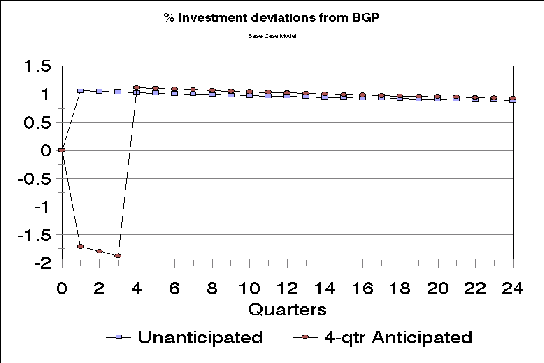
Figure 3 shows a positive anticipation effect in consumption. Again, this is due to intertemporal substitution in anticipation of relatively high consumption in the future. As seen in Figure 4 it is accomplished, despite lower output over the anticipation period, by reductions in the rate of investment. Since consumption rises during the period of anticipation while output falls, a lower correlation between these two variables results and, the relatively smooth path of consumption compared to output implies a lower ratio of standard deviations, $\sigma _{C}/\sigma _{Z}$.

As discussed by Beaudry and Portier (2000) the pattern of variable movements outlined above in response to an anticipated increase in technology is an artifact of the standard RBC model structure employed here. While it is tempting to relate the declines in hours, output, and investment with a recession (in the absence of technological regress), the co-movement of consumption with these variables distinctly contradicts the pattern observed in actual recessions. Clearly anticipation effects cannot make a fully comprehensive model of the business cycle out of the standard RBC structure, and it is not our objective here to argue that. However, as we will see further in the next section, anticipation effects in these models are significant and can address some of their other failures.

3.2 Estimated Autocorrelation and Impulse-Response Functions.

3.2.1 Preliminary Discussion.

Following the methodology of Cogley and Nason (1995) we use our simulated data to calculate estimates of the model's output-growth autocorrelation function and impulse-response functions for output and hours. These estimates are then compared with those obtained from actual time-series data. The objective is to gauge the model's ability to mimic the propagation of shocks that is apparent in the actual time-series.

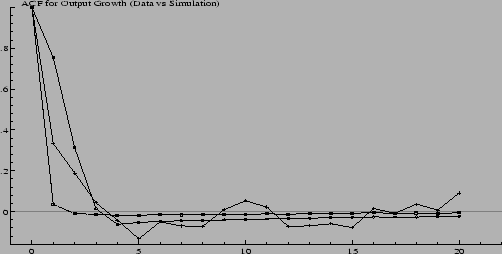
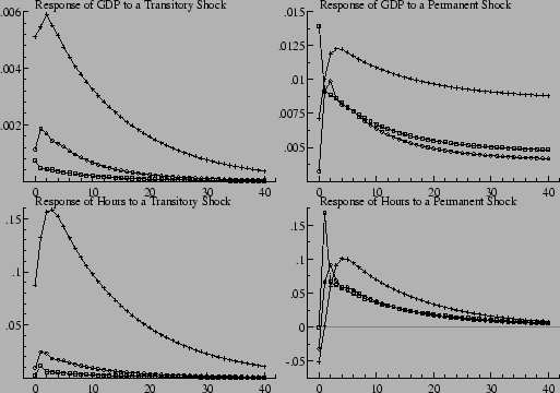
Impulse response functions are estimated employing the methodology of Blanchard and Quah (1989). Given an estimated bivariate autoregressive process obtained from stationary time-series (here quarterly per-capita output growth and hours), this methodology allows for the decomposition of the two variable's responses to shocks into transitory components, which by construction eventually die out, and permanent ones which need not.

Both in the data and in the simulations we use 187 observations corresponding to our sample period of 1954:1 to 2000:3. Estimates reported for the model simulations are the average over the number of replications $(R=1000)$. In all cases we employ a lag length of 8.

Graphical visualisation of the autocorrelation functions and impulse response functions is informative but we also report two statistics for the autocorrelation. The first $(P_{AR_{1}})$ due to Gregory and Smith (1991) gives the probability of observing a first-order autocorrelation coefficient of output growth in the model that is at least as large as that found in the data.

The second $(Q_{acf})$ is discussed by Cogley and Nason (1995). The null hypothesis is that the simulated autocorrelation function is equal to the sample autocorrelation function and thus a low enough $P$-value indicates that the model's autocorrelation function is not a good approximation to the sample autocorrelation functiontypeset@protect @@footnote SF@gobble@opt Further discussion regarding calculation of this statistic is provided in the Appendix C. .

3.2.2 Results.

Figure 5 plots the estimated autocorrelation functions for output growth from the data and from the unanticipated, and 4-quarter anticipated simulations of our base-case model. Consistent with the very poor first-order autocorrelation coefficient estimates given in table 2 above, both models produce very poor estimates of the autocorrelation functions. The reported $P_{AR_{1}}$and$Q_{acf}$ statistics (P-values in parentheses) emphasize this failure. One interesting feature of these plots is the appearance of a downward spike in the autocorrelation function for the 4-quarter anticipated case at lag 3. This clearly reflects the zig-zag path of output in the model, as displayed in Figure 2, in response to the arrival of technological changes 4 periods after the economy's initial response.

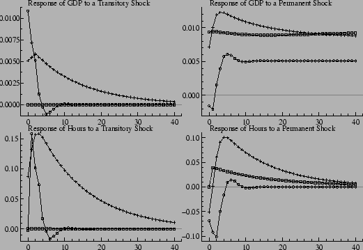
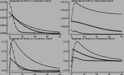
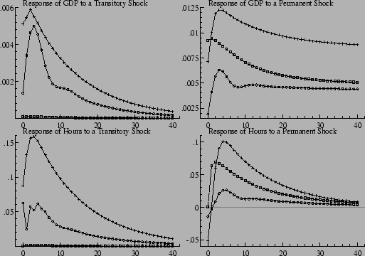
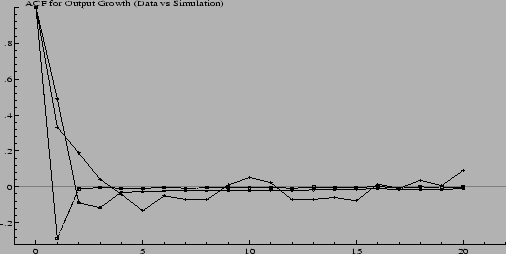
Figure 6 plots the impulse-response functions for output (GDP) and Hours estimated from the data and again, from the unanticipated, and 4-quarter anticipated simulations of our base-case model. As is well known (see, for example, Blanchard and Quah (1989)) the data for both GDP and hours show significant transitory and permanent responses to a shock. Further, each of these responses is characteristically ``hump-shaped''. These facts have proven difficult to replicate with standard RBC models (Cogley and Nason (1995)) and, as shown in Figure 6, the results for our unanticipated case continue to reflect this. The unanticipated case produces virtually no transitory response in either output or hours with the plotted function estimates lying almost entirely along the horizontal axis. While this case does generate permanent responses to a shock these are relatively small and essentially monotonic rather than hump-shaped as for the data.

The 4-quarter anticipated case, on the other hand, displays marked transitory responses in both output and hours. These estimated responses clearly differ from those obtained with the data, nonetheless they indicate an important trend-reverting component in modelled output and hours. Given these sizable transitory responses in the anticipated case, it is not surprising that the decomposition technique employed estimates smaller corresponding permanent responses than found for the unanticipated case. In favourable contrast to the unanticipated case, however, the permanent response functions for the anticipated case are distinctly hump-shaped as is consistent with the non-monotonic permanent responses estimated from the data.

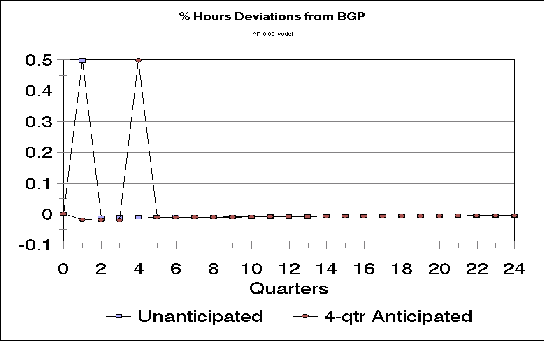
Finally, note that the anticipated case also generates an initial negative response in the permanent hours function which is consistent with the data. This reflects the initial negative response of hours to anticipated future changes in productivity as seen in Figure 1 above. In general, the transitory responses seen when changes in technology are assumed to be anticipated are a reflection of the anticipation effects previously stylized in Figures 1 to 4, which are by their nature short-lived.

4 Alternative Technology Processes in the Base-Case Model.

4.1 Discussion and Model Specification.

It is well known that in large part the stochastic driving processes in RBC models determine the predictions of those models, particularly in regards to propagation mechanisms (see, for example, Cogley and Nason 1993, 1995). We therefore wish to ask how sensitive are our results, regarding the effects of anticipation in RBC models, to the specification of the model's exogenous technological process. In this section then we consider some alternative specifications for the evolution of the model's production technology.

The production function specification in the model is modified to the following;

$$Z_{t}=A_{t}S_{t}K_{t}^{\alpha }l_{t}^{1-\alpha },\; \; where,\; \; A_{t}=(1+\mu )A_{t-1}+\xi _{t}.$$ (8)

As before $S_{t}$ is a random productivity shock but is now specified astypeset@protect @@footnote SF@gobble@opt This specification for the shock process is adopted from Jones, Manuelli, and Siu (2000). ;

$$lnS_{t}=z_{t}-\sigma ^{2}_{\xi }/2(1-\rho ^{2}),\; \; z_{t}=\rho ......},\; \; and,\; \; \xi _{t}\sim \, i.i.d.\, N(0,\sigma _{\xi }^{2})\: \forall t.$$ (9)

The N-step forecast of this stochastic process conditional on $z_{t-1}$ is given by,

$$E[log(S_{t+N})\mid z_{t-1}\}=\rho ^{(N+1)}z_{t-1}-\frac{\sigma _{\xi }^{2}}{2(1-\rho ^{2})},$$ (10)

with conditional variance of,

$$Var[log(S_{t+N})\mid z_{t-1}]=\sigma _{\xi }^{2}\sum ^{N}_{i=0}\rho ^{2i}.$$ (11)

These assumptions imply that $E[S_{t}]=1$ and the model has a well defined BGP. Further, for small$\mu$ and in the limit as $\rho \rightarrow 1$ this model is equivalent to that presented in Section 2 above where we assumed a random walk with drift. Essentially then this model specification enables us to study the implications of the degree of persistence in productivity shocks for our results. Also, for $\rho <1$, productivity shocks are by definition temporary (although potentially very long-lived) relative to the exogenous growth path implied by the evolution of the scale parameter $A_{t}$. There are important implications of this for estimated transitory responses to shocks in the model where, based upon our earlier results, we may expect to see significant effects of anticipation and thus this specification provides emphasis for this point of comparison.

4.2 Simulation Results with Alternative Technology Processes.

4.2.1 Basic RBC Statistics.

Table 3 presents the basic RBC statistics calculated from simulations of the standard unanticipated cases and the 4-quarter anticipated cases of the alternative model under 3 choices of the persistence parameter;$\rho =0.99$, $\rho =0.95$, and $\rho =0.0$. For each value of$\rho$, the table also reports a corresponding value of the parameter$\sigma ^{2}_{\xi }$ which, again, is set so as to approximate the variance of output-growth found in the data for the unanticipated cases. Otherwise calibration is identical here to that given in Table 1, since the balanced-growth properties of the model are unaffected by the specification of the stochastic driving process.

As should be expected the model results for the $\rho =0.99$ case are almost the same as those for the random walk model presented in Section 2 above. As the level of persistence in the shock process diminishes, however, it is apparent that the differences between the unanticipated results and the anticipated results narrows. This effect is consistent across every statistic calculated and continues until, for the $\rho =0.0$ case, there is virtually no difference between the unanticipated and anticipated cases.

The intuition for this result is quite simple. Agent's response in anticipation of future productivity changes is larger the longer lasting the effects of those changes are expected to be. For short-lived changes there is little opportunity to benefit from intertemporal substitution of, for example, labour supply and thus little response in anticipation of the change. This can be seen clearly by observing model impulse response functions. Figure 7 displays, for the $\rho =0.0$ model, the percentage deviations of hours from a deterministic BGP in both the unanticipated and 4-quarter anticipated cases given a positive 1/2 percent productivity shock. Compared to Figure 1 from the earlier random walk model, it is clear how both the anticipation effect and the length of response subsequent to the shock vary with the shock persistence. In the $\rho =0.0$ model, the dominant distinguishing feature between the anticipated and unanticipated cases is the timing of the arrival of the productivity change, and it is apparent how these two cases would be virtually indistinguishable statistically. Similar results are also apparent in regards to output, consumption, and investment responses.

4.2.2 Estimated Impulse Response Functions.

Figures 8 and 9 plot the impulse-response functions for output (GDP) and hours estimated from the data and from the unanticipated, and 4-quarter anticipated simulations of the $\rho =0.95$ and $\rho =0.0$ versions of our alternative model. Two main features of these plots relative to Figure 6 presented earlier for the random walk model are apparent. First, there are no long-run permanent effects of shocks. Second, there are now significant transitory responses to shocks in both the unanticipated and anticipated cases. These results reflect the fact that for $\rho <1$, shocks have no permanent effects relative to the balanced-growth path in the model. With anticipation the responses to a transitory shock are larger in the short-term, reflecting significant anticipation effects of the kind seen previously in Figures 1 to 4. However, these estimated responses are far less drawn out then when the shock is unanticipated. On the other-hand, the estimated responses to a permanent shock are also less drawn out and smaller than in the unanticipated case. Anticipation in these model specifications continues to generate a negative initial response of hours to a permanent shock, however, hump-shaped responses are absent or at least less pronounced.

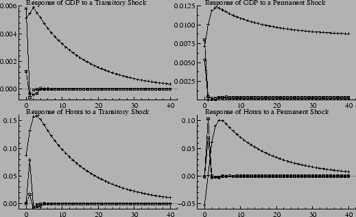
The basic intuition above regarding the implications of persistence for the effects of anticipation in the model extends to the estimated impulse response functions. Figure 9 shows clearly that the estimated response functions in the unanticipated and anticipated cases are essentially the same when the shocks show no persistence $(\rho =0.0)$.

Finally, we do not present estimated autocorrelation functions for these models as there is virtually no change in results. The models all continue to fail miserably in this regard.

5 An Endogenous Growth Model (EGM).

The models examined so far specify long-run growth as an exogenous process. Jones, Manuelli, and Siu (2000) provide a detailed comparison of the business cycle predictions of similar exogenous growth RBC models with a two-sector endogenous growth model (EGM) of human and physical-capital accumulation. They highlight the EGM's persistence properties and, in particular, its ability to generate positive first-order correlation in growth rates of output.

We have seen for exogenous growth models that allowing for anticipation of technology change tends to weaken their (admittedly limited) ability to generate positive persistence in growth rates. Also, our work suggests that the effects of anticipation, particularly with respect to estimated impulse response functions, are sensitive to the assumed growth process. Finally, it is intuitive that allowing for the possibility of intersectoral substitution, as well as for intertemporal substitution, in response to an anticipated technological change may be important for our understanding of business cycles. These factors, and the work of Jones et al. (2000) motivate the analysis in this section of the paper of the effects of anticipation in a two-sector endogenous growth framework.

5.1 Model Specification.

As in Lucas (1988) there are two sectors in the economy: the human-capital sector and the final-goods sector. Human capital is embodied within individuals to provide a supply of ``effective'' labour which is elastically supplied to the market. Each sector employs both this effective labour and physical capital under constant returns to scale. The level of human capital at time t, $H_{t}$, is given by the net accumulation of output from the human-capital sector and physical capital, $K_{t}$, is accumulated by foregoing current consumption from the final-goods sectortypeset@protect @@footnote SF@gobble@opt In addition to Lucas (1988), this class of endogenous growth models has been studied extensively in the growth literature. See for example, Rebello (1991), and King and Rebello (1990). Gomme (1993) examined a monetary version of this model in a RBC context. .

We present here a basic outline of the central remaining features of the model ostensibly for the purposes of establishing notation and a framework for further discussion. Proofs of the existence and uniqueness of competitive equilibrium in this framework, detailed analyses of balanced-growth solutions, and analytical characterizations of the model's transitional dynamic properties are well established elsewhere in the literature. An excellent reference in this regard for readers further interested is Barro and Sala-i-Martin (1996, chpt. 4).

We assume the same utility and information structure for the representative household as given in Section 2.1 above. Time available for leisure $(L_{t})$, however, is now subject to the following constraint;

$$L_{t}=1-l_{Kt}-l_{Ht},$$ (12)

where total hours available have been normalized to unity. $l_{Kt}$ represents hours supplied for employment in the final-goods sector, and $l_{Ht}$ is hours employed in human-capital formation.

The household's effective labour supply $H_{t}(l_{Kt}+l_{Ht})$ earns a competitive wage rate, $w_{t}$. Households also save directly in physical capital which is rented out each period for a competitive rate of return, $r_{t}$. The resulting household income is allocated between the purchase of consumption goods, physical-capital investments, and human-capital accumulationtypeset@protect @@footnote SF@gobble@opt The assumption that human-capital is explicitly purchased in a market rather than, say being produced by households at home, is made for simplicity of exposition only. Under constant returns to scale and perfect competition as assumed here, the results are invariant to this choice. implying the following time-t budget constraint;

$$C_{t}\leq w_{t}H_{t}(l_{Kt}+l_{Ht})+r_{t}K_{t}-(K_{t+1}-(1-\delta _{K})K_{t})-q_{t}(H_{t+1}-(1-\delta _{H})H_{t}).$$ (13)

Here $\delta _{K}\in (0,1)$, and $\delta _{H}\in (0,1)$ give the rates of depreciation of physical-capital and human-capital respectively, and$q_{t}$ gives the relative price of human capital in terms of final-goods.

Final-goods production, $Y_{t}$, is undertaken by firms which employ effective labour and rent proportion $\theta _{t}$ of the capital stock to maximize period-by-period profits. Human capital production, $X_{t}$, employs a symmetric production technology and pays the same wages and rental rates as in the final-goods sector. The corresponding production technologies are;

$$Y_{t}=A_{K}S_{Kt}(\theta _{t}K_{t})^{\alpha }(l_{Kt}H_{t})^{1-\alpha }.$$ (14)

$$X_{t}=A_{H}S_{Ht}((1-\theta _{t})K_{t})^{\gamma }(l_{Ht}H_{t})^{1-\gamma },$$ (15)

Here, $A_{K}>0$, $A_{H}>0$, $\alpha \in (0,1)$, and $\gamma \in (0,1)$ are standard production function coefficients. $S_{Kt}>0$ and $S_{Ht}>0$ are exogenous productivity shocks. For simplicity we will assume that the two sectors are subject to identical shocks in each period so that $S_{Kt}=S_{Ht}=S_{t}\: \forall t$. These shocks are assumed to follow the process given by Equations 9 to 11 in Section 4.1 abovetypeset@protect @@footnote SF@gobble@opt Note that, as opposed to the model of Section 4.1, the rate of growth here is a function of the scale parameters in the constant returns to scale production technologies (i.e. $A_{K}S_{t}$ and $A_{H}S_{t}$). In this version of the model therefore, similarly to the random walk model of Section 2, shocks will by definition have permanent effects. .

The final-goods market-clearing condition is;

$$Y_{t}=C_{t}+K_{t+1}-(1-\delta _{K})K_{t}.$$ (16)

Market clearing in human-capital implies;

$$X_{t}=H_{t+1}-(1-\delta _{H})H_{t}.$$ (17)

Finally, it can be readily shown that the optimal intersectoral allocation of factors implies the following expression for the relative price of human-capital in terms of final-goods output;

$$q_{t}=\frac{\partial Y_{t}/\partial l_{Kt}}{\partial X_{t}/\parti......{\alpha }}{(1-\gamma )A_{H}S_{Ht}((1-\theta _{t})K_{t}/H_{t}l_{Ht})^{\gamma }}.$$ (18)

Employing this condition we calculate aggregate economic output from the model as;

$$Z_{t}=Y_{t}+q_{t}X_{t.}$$ (19)

5.2 Calibration and Measurement in the EGM.

Calibration of this model for the purposes of numerical simulation poses a few additional difficulties over the standard RBC framework due to the explicit modeling of the difficult to measure human-capital sector. As discussed in Jones et al. (2000) some elements of human-capital accumulation are likely attributed to consumption in the data (for example, tuition payments and components of health care). Others are measured in the data as inputs to the production process (research and development, and worker training), while still others are not measured at all (parental input to child rearing, student effort in schooling, and learning-by-doing). Additionally, there is basically no solid evidence regarding the relative factor intensities in production of human capital (determining$\gamma$) or on the rate of depreciation of human capital ($\delta$$_{H}$).

In order to isolate the effects of alternative parameter specifications and/or approaches to measurement on our results we adopt a three-pronged strategy. First we specify a base-case EGM model following a common practice in this framework of assuming perfect symmetry between production sectors (i.e. identical technologies ($A_{K}=A_{H}$ and $\alpha =\gamma$), and depreciation rates ($\delta _{K}=\delta _{H}$)). This amounts to assuming a single-sector model of homogeneous output $(q_{t}=1)$ and consumption goods which therefore, relative to the models of Sections 2 and 4 above, differs essentially only in regards to the endogenous versus exogenous growth assumption.

Second, in the perfectly symmetric sectors EGM the critical ratio of human-to-physical capital is a constant and transitional dynamic responses of the capital stocks to changes in economic conditions transpire within a single time period. Assuming symmetric effects of technology changes between sectors $(S_{Kt}=S_{Ht})$, this implies no intersectoral shifting of resources in response to any given productivity shock, and thus rules out this possible avenue for the effects of anticipation of shocks. We therefore modify the base-case EGM to allow for alternative asymmetries between sectors and examine the implications.

Third we extend the base-case EGM and the asymmetric-sectors models in an attempt to address some of the measurement issues outlined above.

In each case calibration employs the same stylized facts and basic methodology used for the previous models. The specifics of each of these alternative approaches are discussed below in conjunction with the presentation of corresponding results.

5.3 The Base-Case EGM.

Table 4 provides a summary of the parameter settings and corresponding balanced-growth variables for our base-case EGM calibration, and Table 5 presents the corresponding RBC statistics estimated from our simulated data. Results for two choices of persistence parameter $\rho$ are given. Following Gomme (1993) we use $\rho =0.95$. Alternatively, Jones et al. (2000) estimate$\rho =0.95$ for an annual calibration of their model, implying$\rho =0.9877$ for our quarterly version.

Qualitatively the results here are perfectly analogous to those found for the base-case one-sector model studied above. Anticipation raises the variance of output $(\sigma _{Z})$ and of output growth $(\sigma _{g_{Z}})$. $\sigma _{C}/\sigma _{Z}$ falls while $\sigma _{I}/\sigma _{Z}$ and $\sigma _{H}/\sigma _{Z}$ increase under anticipation. The anticipation effect continues to break down the pattern of near perfect correlations of consumption with output $(\rho (C,Z))$, investment with output $(\rho (I,Z))$, and hours with output $(\rho (H,Z))$. Lastly, anticipation worsens the model's already weak predictions regarding the first-order autocorrelations of output growth $(\rho _{1}(g_{Z}))$, and of consumption growth $(\rho _{1}(g_{C}))$. Model impulse response functions for this base-case EGM are also qualitatively identical to those in Figures 1 to 4 from the one-sector models showing the same intuition as was discussed in that case.

Quantitatively, however, these effects are smaller than in the one-sector random walk model and can be seen to diminish with the degree of persistence in the shock process. The base-case EGM clearly shows the same effects of persistence as were seen for the alternative specifications of the one-sector model studied in Section 4 above.

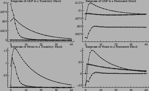
This fact is reiterated in the estimated impulse-response functions for the model shown in Figure 10 for the $\rho =0.9877$ case, and Figure 11 for the $\rho =0.95$ case. As for the one-sector model the base-case EGM shows no transitory responses of either hours or output, but significant transitory responses are estimated in the anticipated case. Correspondingly, permanent responses are estimated to be smaller under anticipation. These estimated impulse response functions are very similar in the $\rho =0.9877$ case to those for the base-case one-sector model where shocks followed a random walk and, in particular, they show a characteristic hump-shaped response. This later property is lost, however, as the shock persistence declines. A comparison with the $\rho =0.95$ case shows reduced responses on the transitory side under anticipation, and permanent responses under anticipation which are getting closer to the of responses seen in the unanticipated case.

These results indicate that endogenizing the growth process in itself has little impact on the nature of the effects of anticipation of productivity shocks for the business cycle predictions of this class of models.

5.4 Asymmetric Sectors.

It may seem unlikely that the processes employed in producing human and physical capital would be perfectly symmetric in terms of relative factor intensities. As stressed by Barro and Sala-i-Martin (1995, chpt. 5), intuition and casual observation suggest the empirically relevant case to be where human-capital production is relatively intensive in the use of human capital. It also seems unlikely that human and physical capital are subject to equal rates of depreciation. Intuition suggests that knowledge capital embodied within individuals is relatively long lived. To address this possibility we specify two alternative models to the base-case EGM.

In the first of these alternatives (EGM-B) we reduce the intensity of physical-capital utilization in the human-capital sector (smaller $\gamma$) by a small margin such that the estimated income share of capital in GDP (and by construction also the share of labour) continues to satisfy the calibration requirements. In the second alternative (EGM-C) we reduce the rate of depreciation on human capital relative to the rate on physical capital. In both of these cases we fix $\rho =0.95$. The corresponding calibrations for these models are given in Tables 8 and 9 found in Appendix D.

Table 6 presents the corresponding RBC statistics estimated from our simulated data. Generally, anticipation of technology change continues to have significant effects. Except where investment is concerned we once again find the same basic pattern of results as for our previous models. In the EGM-B case $\sigma _{I}/\sigma _{Z}$ is still seen to rise with anticipation, however, in the EGM-C case there is a significant fall in this measure relative to the unanticipated case. In both the EGM-B and EGM-C cases we also see a dramatic fall, rather than only a minor one, in the correlation of investment to output$(\rho (I,Z))$ in the anticipated case relative to the unanticipated case.

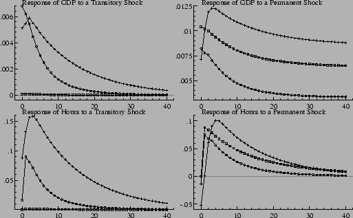
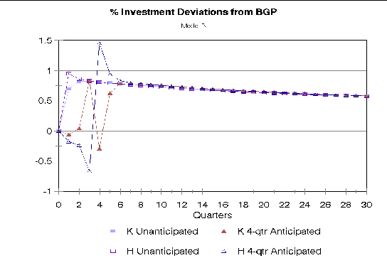
These results can be understood by observing the model impulse response functions. For hours, consumption, and output, these transition paths remain qualitatively identical to those shown for the base-case one-sector model in Figures 1 to 3 above. In these asymmetric sector models, however, since the ratio of human-to-physical capital is no longer constant, but varies in transition, the investment paths for human versus physical-capital, rather than being identical, show markedly different behaviours from each other. Figure 12, shows the paths of human and physical-capital investment in the EGM-B model in response to a 1/2 percent positive productivity shock. In the anticipated case physical-capital investment rises in the periods prior to the technological change, and falls significantly on the arrival date (period 4) before rising again subsequent to the technological change taking effect. Human-capital investment follows an opposite pattern. The movements of physical-capital investment at the arrival date are in the opposite direction to those for output on this date, and being relatively large, this accounts for the models low prediction regarding the correlation of output and physical-capital investment.

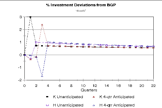
Figure 13 shows that investment deviations in the EGM-C model follow similar paths, although with generally higher volatility than in the EGM-B case which accounts for the increased relative volatility of investment to output in this model. Also, the timing of investment swings differs. This is a reflection of the asymmetries in depreciation rates between sectors which characterizes this model. In the anticipated case, while physical-capital investment is still high in the period before the arrival date, and human-capital investment is low, there is no overshooting of these rates from their long-run levels on the arrival date itself. The transitional responses of investments are essentially completed before the arrival date. This is contrasted with the unanticipated case, where the need to adjust the ratio of capital stocks in response to the arrival of the technological shock forces adjustment on the arrival date itself and accounts for the reduction in the relative volatility of physical-capital investment to output under anticipation.

Finally, estimated impulse-response and autocorrelation functions for these asymmetric cases show almost no variation in results relative to the symmetric sector model and thus are not presented here. There does arise a very small estimated transitory response for both output and hours in the unanticipated cases which verifies the intuition that allowing for intersectoral reallocations of resources in response to shocks may influence the models output dynamics, however, there are no implications for the relative effects of anticipation.

5.5 Alternative Measurements of the Human Capital Sector.

5.5.1 Discussion.

Next we extend our base-case EGM model and the two asymmetric sector cases ``EGM-B'' and ``EGM-C'' in an attempt to address some of the measurement issues outlined above. The only evidence that we are aware of in regards to empirically establishing the extent of mismeasurement (or non-measurement) of human-capital investment in the national accounts is Kendrick (1976, Tables A-1 and B-2). A rough guideline from this work suggests that only one-half of gross investment in human capital is included in measured output. Using this estimate as the fraction ($\lambda$) of human-capital investment not measured in the output data, and given that the share of human-capital investment in aggregate output along a balanced growth path in our base-case model is $q_{t}X_{t}/Z_{t}=0.41$, then the model will be overestimating measured output by roughly 20 percent.

To account for this we adjust our measures of output and incomes earned from the human-capital sector by fraction $\lambda =0.5$. These adjustments have no impact on the actual structure of the model (aside from a need for re-calibration) but only affect how our simulated data series are constructed from the model solutions.

Since some fraction of labour inputs to the human-capital production process are not measured (for example, student hours in school, parental inputs, some portion of time learning-by-doing) we write,

$$Hours_{t}=l_{Kt}+\lambda l_{Ht},$$ where $Hours_{t}$ refers to measured labour hours rather than actual hours worked. Accordingly, a fraction of effective income earned in the production of human capital is not measured. Therefore we write measured labour income as;

$$Linc_{t}=w_{t}H_{t}(l_{Kt}+\lambda l_{Ht}).$$ Similarly we assume that some returns from physical capital in the production of human capital (for example, university and school buildings, publicly run hospitals, museums, etc.) are not measured in the national income accounts. Thus we write measured capital income as:

$$Kinc_{t}=r_{t}K_{t}(\theta _{t}+\lambda (1-\theta _{t})).$$ Finally, we rewrite Equation 19, for measured aggregate output as;

$$Z_{t}=Y_{t}+\mu q_{t}X_{t},$$ (20)

These adjustments do not address the inclusion of human-capital investments in aggregate consumption data. In our view the least ad-hoc method of dealing with this expenditure side measurement issue would be to subtract from the actual consumption data those components which are readily attributed to human-capital accumulation. To this end we deducted personal consumption expenditures on education and research services, and personal consumption expenditures on medical services from our base consumption series for the U.S. We found no appreciable difference in the statistical properties of this series over the base consumption series (besides the reduction in average percentage of GDP) and thus do not report particular results in this regard.

The modification of our models to account for these measurement changes requires alternative calibrations in order to continue to provide variable solutions consistent with observation. By assuming that more hours are actually worked in human-capital accumulation than are measured, total hours in the model must rise for measured hours to match our calibration requirements. The percentage of human-capital output in measured aggregate output falls by roughly one half from 40% of measured aggregate output to 20%, which seems like a more reasonable number. Since physical-capital investment is fully measured in the model, but the measure of aggregate output is now smaller, the $Kinv/Z$ ratio falls unless depreciation rates are lowered.

We refer to these variations of our model as the ``unmeasured'' cases (``Base-Case EGMu'', ``EGMu-B'', ``EGMu-C''). The parameters and balanced-growth variable values for each of these calibrations are given in Tables 10, 11, and 12 found in Appendix D.

5.5.2 Basic RBC Statistics

Table 7, shows the basic RBC statistics generated from our simulations of the ``Base-Case EGMu'', ``EGMu-B'', and ``EGMu-C'' models in both the unanticipated and 4-quarter anticipated cases. Again, a number of variations in the results are apparent in these cases. Generally, there are no implications for the symmetric sector model. This should be expected since, as discussed previously, this symmetry amounts to assuming a single-sector model of homogeneous output and consumption goods with $q_{t}=1$, and therefore the mismeasurement we consider boils down to a uniform rescaling of all of the relevant variables.

In regards to the asymmetric sector cases there are three basic results. First, volatilities of output, and output growth tend to fall with anticipation here rather than rise as we saw in the earlier results. Second, incomplete measurement of the human-capital sector further exacerbates the breakdown in the near perfect correlations between output and consumption, output and investment, and output and hours which results in the anticipated cases. Finally, the ``EGMu-B'' and ``EGMu-C'' cases both show substantial positive autocorrelation of output growth for the case of anticipated technological change. As might be expected then, and as is shown in the next section, these cases also improve significantly on the models predictions for the autocorrelation function of output growth.

5.6 Estimated Autocorrelation and Impulse Response Functions.

As we have seen, mismeasurement of the human-capital sector has virtually no implications in the symmetric sector model. We therefore discuss the estimated autocorrelation and impulse-response functions from the ``EGMu-B'' and ``EGMu-C'' models only (Figures 15, 14, 17, and 16). The message here remains essentially the same as that gained in regards to previous models. Anticipation effects significantly improve predictions with respect to the dynamic properties of output and hours. A large transitory component in the estimated response functions arises under anticipation where none is present when technological change arrives without warning. Additionally, the response functions often display the typical hump-shape found in the data, and improvements in the initial responses of hours worked (i.e. negative values) are also seen. Finally, while the $Q_{acf}$ statistics continue to reject the complete autocorrelation functions estimated for these cases of the model, the $P_{AR_{1}}$statistics confirm strong first-order autocorrelation of output growth when technological change is anticipated. A tentative conclusion from this is that mismeasurement of factors relating to human-capital accumulation may be important for understanding some of the autocorrelation properties seen in the data.

6 Conclusions

This paper explores some of the implications of fully anticipated technological change for the predictions of real business cycle models. Our simulation results show that anticipation of technological change has significant effects on the predictions for various moments of economic data in a wide number of model frameworks. In addition, we estimate impulse-response functions from our simulated data for both output-growth and hours which are roughly consistent with those obtained from US data, and where such responses are basically non-existent in the unanticipated case. In some cases strong autocorrelation of output growth is also predicted when technological changes are anticipated. This suggests that anticipation effects can go some way to providing realistic internal propagation mechanisms within theoretical economic models and to improving our understanding of various economic phenomena including business cycles. This makes sense given the degree to which human behaviour relates to the ability to anticipate events and consequences.

Of course the models fail on some dimensions. Estimated autocorrelation functions are consistently rejected by our calculated Q-statistics relative to the sample functions for example. But the central point, that anticipation is important for the predictions of these models remains valid and we see no reason why this should not extend to other alternative frameworks. Intuitively, actual economies are likely characterized by combinations of anticipated and unanticipated change as well as processes of updating expectations of change with the revelation of new information. We see this as a promising avenue for future research in the RBC literature and elsewhere.

Appendix A. Data.

U.S. quarterly data series employed covered the period 1954:1 to 2000:3. Series denoted in italics where obtained from the National Income and Product Accounts data matrix (NIPAQ) downloaded from the EconData web-site at the University of Maryland. Series denoted in noun-style type where obtained from the Federal Reserve Economic Database (FRED) and where aggregated from monthly to quarterly. Where applicable all series were deflated by the implicit price deflator (d0104), and were divided by the civilian non-institutional population 16 years of age and older (CNP16OV) to obtain per-capita values.

Output figures are gross domestic product (n0101).

Consumption is measured as the sum of, personal consumption expenditure (c0201), Federal government defense expenditures (g0704), Federal government non-defense expenditures (g0715), and State and Local government expenditures (g0728).

Labour income was measured as the sum of, compensation of employees (n1402) and proprietors income with inventory valuation and capital consumption adjustments (n1409).

Capital income was measured as gross national income (n0928) less labour income.

Capital investment was measured by the sum of, private fixed investment (v0401), Federal government defense investment (g0711), Federal government non-defense investment (g0724), and State and Local government investment (g0735).

Our measure of ``hours worked'' accords closely with the Citibase ``Lhours'' series which was not used as it ends at the last month of 1993. Thus we constructed;
 

$$hours = avg.hrs.\times employment\: rate\times participation\: rate$$

$$= avg.hrs.\times employment\div population$$

where avg.hrs. was given by, average weekly hours of production workers (BLS national employment, hours, and earnings series EEU005 annual figures extrapolated to quarterly) for the period 1954:0 to 1963:4, and by average weekly hours of non-agricultural workers (awhnonag) for the period 1964:1 to 2000:3 (monthly data averaged to quarterly). The later series was employed as the former is seasonally unadjusted after 1964. In any case, all of our results appear robust to this choice. Employment was measured by civilian employment 16 years of age and older (CE16OV), and population was again (CNP16OV).

Finally, the labour force was measured by the civilian labour force 16 years of age and older (CLF16OV).

Appendix B. Numerical Simulation.

At the beginning of any time period t, the economy's initial conditions are predetermined by the current value of the state variable $K_{t}$. Also at the beginning of this period we assume that agent's realize the time $t+\tau$ outcome of the stochastic process $\{S_{t}\}$, for some $\tau \geq 0$. Equivalently, at each point in time we have an assumption of perfect foresight for the future period $\{t,...,t+\tau \}$, and the future sequence of technology variables is therefore known for this sub-period. Technology variables for times$\{t+\tau +1,...,T\}$ are forecast conditional on this information, and according to agents' knowledge of the evolution of the stochastic process$\{S_{t}\}$ as given by equations 5 to 7. $T$ gives the possibly infinite length of agents' forecast horizon. A rational expectations forecast for the entire future sequence of technology variables is thus made and a solution for the economy's optimal transitional response in light of this sequence can be calculated by employing standard methodstypeset@protect @@footnote SF@gobble@opt We employ a two-point boundary solution method based on exact specifications of the model's dynamic equations system. As discussed by Fair and Taylor (1984), this imposes the model's terminal conditions improving the efficiency of the solution method. . This expected transition path yields observations for the time t choice variables of the model which determine the time t+1 state variable values. These state variables in turn represent the time t+1 initial conditions for the economy when a new outcome of the stochastic process $\{S_{t}\}$ is realized and thus the basis for a solution of the time t+1 expected transition path is established.

Iteration on the above process Q times yields a Q-period artificial time series for our model economy from which estimates of the moments of the model's variables can be obtained. Following a standard RBC approach (Prescott, 1986), we replicate this entire process R times to generate a large number of such artificial time series and a large sample of estimated moments the averages of which are then compared to real economic data.

In practice we set $T=200$ for the solution of each transition path. This is adequate to ensure that the model converges to its long run balanced growth path with a high degree of numerical accuracytypeset@protect @@footnote SF@gobble@opt Lower values would be adequate with lower persistence in the stochastic process, and correspondingly larger values would be appropriate in the case of greater persistence. . We set Q=200 but truncate the first observations to eliminate any dependence of the simulated series on the $\tau$ starting values. This yields time-series of equal length to our actual data sample (187 observations)typeset@protect @@footnote SF@gobble@opt See Gregory and Smith (1991) for the statistical rational behind requiring equal sample sizes. . Finally we perform R=1000 replications for each model presented.

Appendix C. ACF Statistic.

$Q_{acf}$is computed as,

$$Q_{acf}=(\hat{c}-c)'\hat{V}^{-1}(\hat{c}-c)$$ where $\hat{c}$ and $c$ are $8\times 1$ vectors containing the autocorrelations for the sample and the simulations respectively. The middle term is a covariance matrix calculated as,

$$\hat{V}=\{\frac{1}{R}\}\sum _{i}^{R}(c_{i}-c)(c_{i}-c)'$$ where $c$ is computed as,

$$c=\{\frac{1}{R}\}\sum _{i=1}^{R}c_{i}$$ and $c_{i}$ is the autocorrelation function obtained from replication $i$.$Q_{acf}$ is distributed as a $\chi ^{2}(8)$.

This type of statistic can also be computed for the impulse-response functions if the number of shocks in the model is as large as the order of the vector autoregression (here, two). In the present paper, however, there is only one shock (applied symmetrically to both sectors in the endogenous growth model) and hence the $Q$ statistics for the impulse-response functions are not available.

Bibliography

5

Barro, Robert J., and Xavier Sala-i-Martin, Economic Growth, McGraw-Hill Advanced Series in Economics, 1995.

16

Beaudry, Paul, and Franck Portier, ``An Exploration into Pigou's Theory of Cycles'', University of British Columbia mimeo, November 2000.

5

Blanchard, Olivier Jean, and Danny Quah, ``The Dynamic Effects of Aggregate Demand and Supply Disturbances'', American Economic Review, Vol. 79, Number 4, (Sept. 1989): 655-673.

9

Cogley, Timothy, and James M. Nason, ``Impulse Dynamics and Propagation Mechanisms in a Real Business Cycle Model'', Economics Letters, December 1993, 43(4), pp. 77-81.

5

Cogley, Timothy, and James M. Nason, ``Output Dynamics in Real-Business-Cycle Models'', American Economic Review, Vol. 85, Number 3, (June 1995): 492-511.

8

Christiano, Lawrence J. and Martin Eichenbaum, ``Current Real-Business-Cycle Theories and Aggregate Labor-Market Fluctuations'', American Economic Review, June 1992, 82(3), pp. 430-50.

9

Fair, R. C., and Taylor J.B., ``Solution and Maximum Likelihood Estimation of Dynamic Nonlinear Rational Expectations Models'', Econometrica, 51, (1983): 1169-1185.

8

Gagnon, Joseph E., ``Solving the Stochastic Growth Model by Deterministic Extended Path'', Journal of Business & Economic Statistics'', Vol. 8, No. 1, (January 1990).

9

Gomme, Paul, ``Money and Growth Revisited'', Journal of Monetary Economics, 32, (1993): 51-77

16

Gregory, Allan W., and Gregor W. Smith, ``Calibration as Testing: Inference in Simulated Macroeconomic Models'', Journal of Business and Economic Statistics, Vol. 9, No. 3, (July 1991).

16

Jones, Larry E., Rodolfo E. Manuelli, and Henry E. Siu., ``Growth and Business Cycles'', NBER WP. #W7633, April 2000.

12

Kendrick, John W. The Formation and Stocks of Total Capital, New York, Columbia University Press, 1976.

18

King, Robert G., and Sergio T. Rebelo. ``Public Policy and Economic Growth: Developing Neoclassical Implications.'' Journal of Political Economy 98, (1990): S126-50

14

Lucas, Robert E., ``On the Mechanics of Economic Development'', Journal of Monetary Economics, vol. 22, (1988).

15

Mehra, Rajinish and Edward C. Prescott, ``The Equity Premium: A Puzzle'', Journal of Monetary Economics, 15, (1985), pp. 145-61.

16

Prescott, Edward C. ``Theory Ahead of Business Cycle Measurement'' Carnegie-Rochester Conference Series on Public Policy, 25, (Autumn 1986): 11-44.

17

Rebelo, S.T. ``Long-run Policy Analysis and Long-run Growth'', Journal of Political Economy, 99, (1991): 500-21.

18

Taylor, J.B., and Uhlig, H., ``Solving Nonlinear Stochastic Growth Models: A Comparison of Alternative Solution Methods'', Journal of Business and Economic Statistics, 8, (1990): 1-17.

Table 1: Parameters and Balanced-Growth Variables: Base-Case Calibration

Model Parameters.

$A=1.0$, $\alpha =0.35$, $\delta =0.024$

$\beta =0.987$, $\varepsilon =0.22$, $\sigma =4.0$, $IES=0.6024$

$\sigma _{\xi }=0.0083$, $\mu =0.0027$

Balanced-Growth Variable Values

$g=0.0042$, $l=0.191$

$Kinc/Z=0.35$, $Kinv/Z=0.222$, $r-\delta =0.02$

 

Table 2: Volatilities and Cross-Correlations: U.S. Data, Unanticipated Base-Case model, and 4-period Anticipated Base-Case Model. Logged and Hodrick-Prescott Filtered Data.

	U.S. Data	Unanticipated	4-qtr Anticipated
$\sigma _{g_{Z}}$	0.0095	0.0095	0.014
$\sigma _{Z}$	1.62	1.21	1.61
$\sigma _{C}/\sigma _{Z}$	0.63	0.76	0.37
$\sigma _{I}/\sigma _{Z}$	2.34	1.85	3.91
$\sigma _{H}/\sigma _{Z}$	0.78	0.198	0.68
$\rho (C,Z)$	0.85	0.998	0.58
$\rho (I,Z)$	0.91	0.996	0.96
$\rho (H,Z)$	0.87	0.982	0.93
$\rho _{1}(g_{Z})$	0.33	0.011	-0.007
$\rho _{1}(g_{C})$	0.16	0.03	-0.003

Notation: $\sigma _{x}$ gives the standard deviation of variable x. $\rho (x,y)$ gives the correlation of variables $x$ and $y$. $\rho _{1}(x)$ gives the first-order autocorrelation of variable$x$. $Z$ denotes aggregate output, and $g_{Z}$ its growth rate.$C$ denotes consumption, and $g_{C}$ its growth rate. $I$ denotes capital investment, and $H$ total hours.

Figure 1: Transitional Dynamic Response of Hours.

Figure 2: Transitional Dynamic Response of Output

Figure 3: Transitional Dynamic Response of Consumption

Figure 4: Transitional Dynamic Response of Investment

Figure 5: Estimated Autocorrelation Functions, Data and Base-Case Model.

$P^{Un}_{AR_{1}}=0.0$, $Q_{acf}^{Un}=35.1\: (P=0.00003)$:$P^{An}_{AR_{1}}=0.0$, $Q_{acf}^{An}=52.4\: (P=0.0)$. 

$+-$U.S. data, $\sqcap$ - Unanticipated, $\circ -$4-qtr Anticipated 

Figure 6: Estimated Impulse-Response Functions, Data and Base-Case Model.

Quarters
$+-$U.S. data, $\sqcap$ - Unanticipated, $\circ -$4-qtr Anticipated 

Table 3: Volatilities and Cross-Correlations: U.S. Data, and Section 4 alternative models, Unanticipated, and 4-period Anticipated Simulations. Logged and Hodrick-Prescott Filtered Data.

	Data	$\rho =0.99$	$\sigma ^{2}_{\xi }=.0075$	$\rho =0.95$	$\sigma ^{2}_{\xi }=.007$	$\rho =0.0$	$\sigma ^{2}_{\xi }=.005$
		Un	An	Un	An	Un	An
$\sigma _{g_{Z}}$	0.0095	0.0093	0.013	0.0098	0.012	0.0115	0.0116
$\sigma _{Z}$	1.62	1.19	1.47	1.25	1.40	0.783	0.785
$\sigma _{C}/\sigma _{Z}$	0.63	0.64	0.35	0.48	0.31	0.24	0.23
$\sigma _{I}/\sigma _{Z}$	2.34	2.29	3.77	2.88	3.62	3.66	3.69
$\sigma _{H}/\sigma _{Z}$	0.78	0.3	0.65	0.44	0.61	0.619	0.623
$\rho (C,Z)$	0.85	0.995	0.696	0.982	0.856	0.98	0.987
$\rho (I,Z)$	0.91	0.995	0.972	0.99	0.987	0.999	0.999
$\rho (H,Z)$	0.87	0.985	0.951	0.986	0.977	0.998	0.999
$\rho _{1}(g_{Z})$	0.33	0.0086	-0.0087	-0.012	-0.023	-0.491	-0.492
$\rho _{1}(g_{C})$	0.16	0.041	0.024	0.04	0.032	-0.479	-0.485

Notation: $\sigma _{x}$ gives the standard deviation of variable x. $\rho (x,y)$ gives the correlation of variables $x$ and $y$. $\rho _{1}(x)$ gives the first-order autocorrelation of variable$x$. $Z$ denotes aggregate output, and $g_{Z}$ its growth rate.$C$ denotes consumption, and $g_{C}$ its growth rate. $I$ denotes capital investment, and $H$ total hours.

Figure 7: Transitional Dynamic Response of Hours, $\rho =0.0$ Alternative Model.

Figure 8: Estimated Impulse-Response Functions, Data and $\rho =0.95$ Model.

Quarters
$+-$U.S. data, $\sqcap$ - Unanticipated, $\circ -$4-qtr Anticipated 

Figure 9: Estimated Impulse-Response Functions, Data and $\rho =0.0$ Model.

Quarters
$+-$U.S. data, $\sqcap$ - Unanticipated, $\circ -$4-qtr Anticipated 

Table 4: Parameters and Balanced-Growth Variables: Base-Case EGM Calibration

Model Parameters.

$A_{K}=A_{H}=0.2476$, $\alpha =\gamma =0.35$, $\delta _{K}=\delta _{H}=0.024$

$\beta =0.987$, $\varepsilon =0.1175$, $\sigma =6.8$, $IES=0.59$

$\sigma _{\xi }=0.008$, $\rho =0.95\; or\; 0.9877$

Balanced-Growth Variable Values

$g=0.0042$, $l_{K}=0.113$,$l_{K}+l_{H}=0.192$

$Kinc/Z=0.35$, $Kinv/Z=0.223$, $r-\delta _{K}=0.02$

 

Table 5: Volatilities and Cross-Correlations: U.S. Data, Unanticipated Base-Case EGM, and 4-period Anticipated Base-Case EGM. Logged and Hodrick-Prescott Filtered Data.

	U.S. Data	$\rho =0.95$	case	$\rho =0.9877$	case
		Un	An	Un	An
$\sigma _{g_{Z}}$	0.0095	0.0107	0.012	0.0092	0.012
$\sigma _{Z}$	1.62	1.36	1.44	1.17	1.39
$\sigma _{C}/\sigma _{Z}$	0.63	0.52	0.42	0.73	0.46
$\sigma _{I}/\sigma _{Z}$	2.34	1.28	1.34	1.15	1.36
$\sigma _{H}/\sigma _{Z}$	0.78	0.398	0.49	0.22	0.53
$\rho (C,Z)$	0.85	0.993	0.97	0.999	0.84
$\rho (I,Z)$	0.91	0.999	0.999	0.999	0.994
$\rho (H,Z)$	0.87	0.992	0.986	0.992	0.92
$\rho _{1}(g_{Z})$	0.33	-0.012	-0.015	0.012	0.003
$\rho _{1}(g_{C})$	0.16	0.018	0.0084	0.13	0.004

Notation: $\sigma _{x}$ gives the standard deviation of variable x. $\rho (x,y)$ gives the correlation of variables $x$ and $y$. $\rho _{1}(x)$ gives the first-order autocorrelation of variable$x$. $Z$ denotes aggregate output (equation 19 from the model), and $g_{Z}$ its growth rate. $C$ denotes final-goods consumption, and $g_{C}$ its growth rate. $I$ denotes physical-capital investment, and $H$ total hours $(l_{K}+l_{H})$.

Figure 10: Impulse-Response Functions, Data and Base-Case EGM $\rho =0.9877$.

Quarters
$+-$U.S. data, $\sqcap$ - Unanticipated, $\circ -$4-qtr Anticipated 

Figure 11: Impulse-Response Functions, Data and Base-Case EGM $\rho =0.95$.

Quarters
$+-$U.S. data, $\sqcap$ - Unanticipated, $\circ -$4-qtr Anticipated 

Table 6: Volatilities and Cross-Correlations: U.S. Data, ``EGM-B'' and ``EGM-C'' Unanticipated, and 4-period Anticipated Models. Logged and Hodrick-Prescott Filtered Data.

	Data	EGM-B	Case	EGM-C	Case
		Un	An	Un	An
$\sigma _{g_{Z}}$	0.0095	0.0106	0.012	0.0109	0.012
$\sigma _{Z}$	1.62	1.35	1.43	1.38	1.47
$\sigma _{C}/\sigma _{Z}$	0.63	0.52	0.42	0.49	0.40
$\sigma _{I}/\sigma _{Z}$	2.34	1.20	1.36	3.16	2.52
$\sigma _{H}/\sigma _{Z}$	0.78	0.40	0.49	0.41	0.5
$\rho (C,Z)$	0.85	0.99	0.97	0.99	0.97
$\rho (I,Z)$	0.91	0.99	0.19	0.67	0.047
$\rho (H,Z)$	0.87	0.99	0.98	0.99	0.987
$\rho _{1}(g_{Z})$	0.33	-0.015	-0.02	-0.007	-0.016
$\rho _{1}(g_{C})$	0.16	0.014	-0.01	0.017	0.0026

Notation: $\sigma _{x}$ gives the standard deviation of variable x. $\rho (x,y)$ gives the correlation of variables $x$ and $y$. $\rho _{1}(x)$ gives the first-order autocorrelation of variable$x$. $Z$ denotes aggregate output (equation 19 from the model), and $g_{Z}$ its growth rate. $C$ denotes final-goods consumption, and $g_{C}$ its growth rate. $I$ denotes physical-capital investment, and $H$ total hours $(l_{K}+l_{H})$.

Figure 12: Transitional Dynamic Responses of Capital Investments: ``EGM-B''.

Figure 13: Transitional Dynamic Responses of Capital Investments: ``EGM-C''.

Table 7: Volatilities and Cross-Correlations: U.S. Data, ``Base-Case EGMu'', ``EGMu-B'', ``EGMu-C'' Unanticipated , and 4-period Anticipated Models. Logged and Hodrick-Prescott Filtered Data.

	Data	Base-Case	EGMu	``EGMu-B''& case	``EGMu-C''& case
		Un	An	Un	An	Un	An
$\sigma _{g_{Z}}$	0.0095	0.0097	0.104	0.0093	0.005	0.0015	0.0073
$\sigma _{Z}$	1.62	1.247	1.28	1.22	1.04	1.453	1.168
$\sigma _{C}/\sigma _{Z}$	0.63	0.496	0.41	0.51	0.51	0.42	0.44
$\sigma _{I}/\sigma _{Z}$	2.34	1.68	1.8	1.56	3.43	3.54	3.64
$\sigma _{H}/\sigma _{Z}$	0.78	0.365	0.434	0.35	0.41	0.51	0.48
$\rho (C,Z)$	0.85	0.99	0.97	0.99	0.92	0.942	0.91
$\rho (I,Z)$	0.91	0.998	0.997	0.98	0.20	0.86	0.48
$\rho (H,Z)$	0.87	0.994	0.987	0.99	0.80	0.945	0.87
$\rho _{1}(g_{Z})$	0.33	-0.017	-0.02	0.003	0.73	-0.29	0.47
$\rho _{1}(g_{C})$	0.16	-0.006	-0.004	0.004	-0.02	0.006	-0.006

Notation: $\sigma _{x}$ gives the standard deviation of variable x. $\rho (x,y)$ gives the correlation of variables $x$ and $y$. $\rho _{1}(x)$ gives the first-order autocorrelation of variable$x$. $Z$ denotes aggregate output (equation 20 from the model), and $g_{Z}$ its growth rate. $C$ denotes final-goods consumption, and $g_{C}$ its growth rate. $I$ denotes physical-capital investment, and $H$ total hours $(l_{K}+\lambda l_{H})$.

Figure 14: Estimated Autocorrelation Functions, Data and ``EGMu-B''.

$P^{Un}_{AR_{1}}=0.0$, $Q_{acf}^{Un}=27.49\: (P=0.0006)$:$P^{An}_{AR_{1}}=1.0$, $Q_{acf}^{An}=47.5\: (P=0.0)$. 

$+-$U.S. data, $\sqcap$ - Unanticipated, $\circ -$4-qtr Anticipated

Figure 15: Estimated Impulse-Response Functions, Data and ``EGMu-B''

Quarters
$+-$U.S. data, $\sqcap$ - Unanticipated, $\circ -$4-qtr Anticipated 

Figure 16: Estimated Autocorrelation Functions, Data and ``EGMu-C''.

$P^{Un}_{AR_{1}}=0.0$, $Q_{acf}^{Un}=34.0\: (P=0.00004)$:$P^{An}_{AR_{1}}=0.99$, $Q_{acf}^{An}=54.7\: (P=0.0)$. 

$+-$U.S. data, $\sqcap$ - Unanticipated, $\circ -$4-qtr Anticipated 

Figure 17: Estimated Impulse-Response Functions, Data and ``EGMu-C''.

Quarters
$+-$U.S. data, $\sqcap$ - Unanticipated, $\circ -$4-qtr Anticipated 

Appendix D. Asymmetric Sectors and ``Unmeasured'' - case Calibrations.
 
 

Table 8: Parameters and Balanced-Growth Variables: EGM-B 

Model Parameters

$A_{K}=A_{H}=0.2493$, $\alpha =0.35$, $\gamma =0.34$, $\delta _{K}=\delta _{H}=0.024$

$\beta =0.987$, $\varepsilon =0.1166$, $\sigma =6.8$, $IES=0.6$

$\sigma _{\epsilon }=0.008$, $\rho =0.95$

Balanced-Growth Variable Values

$g=0.0042$, $l_{K}=.111$, $l_{K}+l_{H}=0.192$

$Kinc/Z=0.346$, $Kinv/Z=0.22$, $r-\delta _{K}=0.02$

 

Table 9: Parameters and Balanced-Growth Variables: ``EGM-C''.

Model Parameters

$A_{K}=A_{H}=0.227$, $\alpha =\gamma =0.35$, $\delta _{K}=0.024,\; \delta _{H}=0.018$

$\beta =0.987$, $\varepsilon =0.129$, $\sigma =6.8$, $IES=0.57$

$\sigma _{\epsilon }=0.008$, $\rho =0.95$

Balanced-Growth Variable Values

$g=0.0042$, $l_{K}=.12$, $l_{K}+l_{H}=0.192$

$Kinc/Z=0.35$, $Kinv/Z=0.221$, $r-\delta _{K}=0.02$

 

Appendix D, Continued.
 
 

$$\lambda =0.5$$

Table 10: Parameters and Balanced-Growth Variables: ``Base-Case EGMu''

Model Parameters

$A_{K}=A_{H}=0.1724$, $\alpha =\gamma =0.35$, $\delta _{K}=\delta _{H}=0.014$

$\beta =0.987$, $\varepsilon =0.181$, $\sigma =5.4$, $IES=0.56$

$\sigma _{\epsilon }=0.008$, $\rho =0.95$

Balanced-Growth Variable Values

$g=0.0042$, $l_{K}=.153$, $l_{K}+\lambda l_{H}=0.192$

$Kinc/Z=0.35$, $Kinv/Z=0.22$, $r-\delta _{K}=0.02$

 

$$\lambda =0.5$$

Table 11: Parameters and Balanced-Growth Variables: ``EGMu-B'' Model 

Model Parameters

$A_{K}=A_{H}=0.173$, $\alpha =0.35$, $\gamma =0.34$, $\delta _{K}=\delta _{H}=0.014$

$\beta =0.987$, $\varepsilon =0.1808$, $\sigma =5.4$, $IES=0.56$

$\sigma _{\epsilon }=0.008$, $\rho =0.95$

Balanced-Growth Variable Values

$g=0.0042$, $l_{K}=.152$, $l_{K}+\lambda l_{H}=0.192$

$Kinc/Z=0.348$, $Kinv/Z=0.218$, $r-\delta _{K}=0.02$

 

$$\lambda =0.5$$

Table 12: Parameters and Balanced-Growth Variables: ``EGMu-C'' Model 

Model Parameters

$A_{K}=A_{H}=0.1639$, $\alpha =\gamma =0.35$, $\delta _{K}=0.014,\; \delta _{H}=0.0105$

$\beta =0.987$, $\varepsilon =0.188$, $\sigma =5.4$, $IES=0.55$

$\sigma _{\epsilon }=0.008$, $\rho =0.95$

Balanced Growth Variable Values

$g=0.0042$, $l_{K}=.158$, $l_{K}+\lambda l_{H}=0.192$

$Kinc/Z=0.35$, $Kinv/Z=0.215$, $r-\delta _{K}=0.02$

About this document ...

This document was generated using the LaTeX2HTML translator Version 99.2beta6 (1.42)

Copyright © 1993, 1994, 1995, 1996, Nikos Drakos, Computer Based Learning Unit, University of Leeds.
Copyright © 1997, 1998, 1999, Ross Moore, Mathematics Department, Macquarie University, Sydney.

The command line arguments were:
latex2html -no_subdir -split 0 -show_section_numbers /home/loved/Working/Papes/RBCgrow/RBCAnt-v3.tex

The translation was initiated by David Love on 2001-10-27